Introduction
Some Initial Thoughts on Algorithmic Composition
Intuition
Repetition at a steady rate
Tempo-relative timing
Timed Counting
Counting through a List
Analysis of Some Patterns
That's Why They Call Them Digital Media
Linear change
Fading by means of interpolation
Randomness
Randomness and noise
Limiting the range of random choices
Moving range of random choices
A simple probabilistic decision
Probability distribution
Line-segment control function
Control function as a recognizable shape
Classic waveforms as control functions
Sine wave as control function
Pulse wave, a binary control function
Triangle wave as a control function
Discrete steps within a continuous function
First steps in modulating the modulator
Second steps in modulating the modulator
Modulating the modulators
Some Initial Thoughts on Visualizing Music
Thursday, September 24, 2009
Some Initial Thoughts on Visualizing Music
The variety of possible relationships between sound and image is a vast and intriguing subject. In terms of visualizing music, it can include music notation, spectrographic displays, paintings inspired by music, son et lumière, software that algorithmically generates animation based on sound, music videos, Schenkerian analyses, and so on. In terms of "sonifying" images there is music based on paintings, film music, music generated by drawing on film soundtrack, and a wide range of applications of sound used to display numerical data.
Traditional Western music notation attempts to visualize music by means of a symbolic language. Fluent readers of music notation can use it to recreate -- mentally and/or on an instrument -- the music described by that notation. However, such notation does not really try to give a visual analog of the music. Music notation systems are usually intended to a) give a performer a symbolic representation of some aspects of the music's structure and b) give an instructional tablature of how to produce the desired music on an instrument. The distinction between a and b is perhaps best illustrated by music for lute and guitar, which can be written as notes in standard notation or as fingerings in tablature. Notes are better for revealing the musical structure; fingerings are better for revealing the actions required to produce the sound on the instrument. To a greater or lesser degree, each of those two methods of notation serves both functions of description and instruction. But notation is in some ways incomplete and imprecise, and relies on a good deal of unstated cultural knowledge possessed by the reader -- particularly in its treatment of subtleties of timbre, dynamics, rubato, ornamental inflections, etc. Western notation is relatively precise in describing the pitch and rhythm of note events, but is less precise in visualizing the other parameters of musical structure or sonic content.
Digital audio workstation software provides a static amplitude-over-time graph of the sound wave itself. If one zooms in to look closely at a few milliseconds of the sound, one might be able to tell from the waveform whether the sound is periodic, approximately how rich in harmonics it is, or approximately how noisy it is, but since you're only viewing a tiny time segment of the sound, it's hard to know much of interest about its musical content. If one zooms out to look at several seconds of sound one can see its overall amplitude envelope and may thus be able to discern something about its loudness and rhythm, but details of its content are not apparent. It's an adequate visualization for recognizing significant events in the sound and for editing the sound accordingly, but is otherwise not very rich in information.
Likewise a spectrographic display, even an animated one that updates continually in real time, provides information about the frequency content, its harmonicity, inharmonicity, and noisiness, but still requires expert and painstaking analysis and interpretation to derive information about the musical structure.
The following discussion and example will focus on one particular type of visualization: using information derived from the sound or musical structure itself to generate an animation that displays and elucidates one or more aspects of the sonic/musical structure. In other words, visualization that is concerned not with creating an aesthetic object inspired by the music, but with displaying useful information for "understanding" or analyzing the sound.
To visualize music (as distinguished from visualizing sound), we need to focus on the musical attributes that are of particular interest for our purpose. The parameters most important for analyzing music can be many and varied, may be subject of disagreement, and may change as the music proceeds. There are the standard accepted fundamental musical parameters such as pitch, loudness, and duration, some more complex or derived parameters of musical sounds such as timbre, accent, and articulation, and more global attributes of a musical structure such as rhythmic patterns, tempo, event density, dissonance, spatial distribution, and so on. One way to think about music is as an evolving multidimensional entity, in which each dimension corresponds to a parameter or trait or attribute of interest.
How can you depict multi-dimensionality in a two-dimensional space? In addition to the obvious two dimensions, horizontal and vertical, we might consider the color, size, brightness, and shape of objects to be additional dimensions that can carry information. Three-dimensional graphics can give the impression of a third spatial dimension. The passage of time in the visualization generally will correspond to the musical time in a realtime depiction, but other relationships such as slowed-down time or frozen time might also be useful in some circumstances.
The designer/programmer of the visualization must decide what visual dimensions and characteristics most effectively convey musical attributes. For example, we say that pitches are "high" or "low", so we often find it best to depict pitch height in the vertical dimension. On the other hand, we know that in fact there's nothing inherently spatially higher or lower about one pitch relative to another. In some cases we might just as usefully map them to the horizontal dimension, as they appear on a piano keyboard, or to some other continuum. For some synesthetes with perfect pitch, pitch classes might correspond to particular hues. In a particular tuning system or scale system, pitches may be thought of as residing on a virtual grid. There might also be cases in which higher pitches might be deemed more intense or brighter, or lower pitches might be deemed darker or weightier. In short, mappings of sonic and musical attributes to visual dimensions and characteristics are quite subjective and case-dependent, even though many standard mappings exist.
In the program demonstrating counting through a list, one part of the program reads repeatedly through a list of sixteen MIDI pitch numbers. Another part of the program reads through a list of sixteen x,y locations for the display of a black dot. The mapping between the pitches and the dot locations is imprecise, but is still very suggestive of a correlation because the vertical height of the dot corresponds to the pitch height, so the dot seems to depict the pitch contour. The horizontal locations of the dot do not correspond to any specific parameter in the music, but they are chosen so as to suggest a generally circular pattern, thus enhancing the cyclic feeling of the pitch movement when the program counts repeatedly in a loop.
In the programs that demonstrate limiting and moving ranges of random values, pitch is again displayed in the vertical dimension as individual slider positions in a multislider object, and the image is scrolled continuously in the horizontal dimension to depict the passage of time and show the most recent several seconds' worth of note choices.
It's worth noting that in those examples the tempo and rhythm are constant, and are thus not of particular musical interest, so they are not displayed. The dynamics (the note velocities) are of some interest, but arguably of less interest than the pitches, so for the sake of simplicity there's no attempt to display that parameter either.
In the programs that show the first and second steps in modulating the modulator, the pitch of the sound changes in a continuous glissando instead of in discrete steps of the equal-tempered scale, so the pitch value is displayed in a scope~ object capable of displaying the (most recently played one second of the) pitch contour.
The program called "modulating the modulators" produces a sound in which a few different musical attributes are constantly and gradually changing. In that example it's pretty clear what's worth depicting in the sound, because we know what's being modified: the pitch, the volume and the panning (the left-right location). We know this because the computer itself is generating the sound, and we have access to the information that controls those particular parameters. These three parameters can be mapped to three dimensions or characteristics of an animated image.
Here is an example of one possible visualization of the pitch, volume, and panning of the sound generated in the "modulating the modulators" program. (The drawing objects are hidden in the program, but they're shown here in the graphic below.)
.jpg)
This program displays each musical note in terms of its most important attributes: its pitch contour, loudness, and panning. Pitch is shown in the vertical dimension, panning is shown in the horizontal dimension, and volume is shown in terms of the brightness of the note. Since the sound has only a single timbre, it seems reasonable to use a single color to draw the notes. These attributes change during the course of a single note, so the graphic display ends up being a line drawing that depicts the shape of those attributes during the note.
The fragment of the program shown in the picture above has three main focal points: the part that draws the image, the part that stores the image to be drawn, and the part that erases the previously drawn image at the start of each new note.
The drawing part consists of a metro object, a jit.matrix object named notes, and a jit.pwindow object. The dimensions of the jit.pwindow are 128x128 pixels, the same as the dimensions of the jit.matrix. The time interval of the metro is defined such that it will cause the contents of the jit.matrix to be drawn in the jit.pwindow 30 times per second, which is sufficiently often to give a sense of continuity to the animation. The metro gets turned on and off automatically at the same time as the audio is turned on and off, so it's always drawing whenever the sound is playing.
The jit.matrix object is being filled by a jit.poke~ object that refers to the same space in memory. The arguments of jit.poke~ indicate the name of the jit.matrix into which to poke signal values, the number of dimensions of the matrix that we want to access, and the plane number we want to access. (Plane 2 is the green color plane in a 4-plane char ARGB matrix; we're only using the color green.) The purpose of jit.poke~ is to use MSP signals to specify the values and locations to be drawn into the specified plane of the specified matrix. The inlets are, in order from left to right, for the value that will be stored (the brightness of green), the cell location in dimension 0 (the horizontal cell location), and the cell location in dimension 1 (the vertical cell location). The inlets are fed by signals that control volume, panning, and pitch -- the three musical attributes we want to depict. So volume is mapped to brightness, panning is mapped to horizontal location, and pitch is mapped to vertical location. The 128 vertical pixels are mapped to the 0-127 range of MIDI. The signal is first passed through a !-~ 127 object to create an inverse mapping of pitch to pixel number. That's because MIDI pitch values go up from 0 to 127 but cell indices in the matrix go down from 0 to 127. The panning value, which is originally expressed in the range 0 to 1 gets passed through a *~ 127 object to expand it to the horizontal range of the matrix, a range which was chosen for no other reason than to make it the same size as the vertical range. The volume value is originally in the range from 0 to -30 dB, so before it gets to jit.poke~ it gets multiplied by 0.03 to reduce its range to 0 to -0.9, and then has 1.0 added to it to yield brightness values that vary from 1.0 down to 0.1. The result of all of this is that the brightness value that corresponds to volume gets placed into plane 2 of every cell of the matrix that corresponds to a pitch and panning combination that occurs during a given note.
What I'm calling a "note" in this context is each time an amplitude envelope window is generated by the triangle function that modulates the amplitude of the signal coming directly out of the tri~ object in the synthesis patch. Those amplitude envelopes are controlled by the phasor~ that reads through just the first half of the triangle wave function stored in the buffer~. In the drawing portion of the patch you can see the use of the delta~ object to monitor the change in the signal coming from the phasor~. Since the phasor~ generates an upward ramp that goes cyclically from 0 to (almost) 1 and then leaps back to 0, there is a very specific moment, which occurs only at the beginning of each cycle, when the change in the phasor~, instead of being a slight increase, is suddenly a decrease (on the sample when it leaps back to 0). So you can use the <~ 0. object to detect when the change occurs, namely at the instant when delta~ outputs a negative sample value. At that moment the <~ 0. object will output a 1 (the only time the test succeeds), and the edge~ object will report that it occurred. That report is used to trigger a clear message to jit.matrix, causing it to set all its values to 0, effectively erasing the previous note from the matrix.
So in this example, the drawing rate or "refresh" rate of the visual display is 30 times per second, and the content of the display matrix is erased (reset to all 0) once per note. The passage of time is not displayed as a dimension in its own right, but rather by the constant updating of the display. The display changes according to the changing shape of the line being drawn as determined by the change in pitch and panning in the course of each note. This is a non-traditional way to display information about the musical structure, but it directly addresses the three main musical features of this particular sound.
Traditional Western music notation attempts to visualize music by means of a symbolic language. Fluent readers of music notation can use it to recreate -- mentally and/or on an instrument -- the music described by that notation. However, such notation does not really try to give a visual analog of the music. Music notation systems are usually intended to a) give a performer a symbolic representation of some aspects of the music's structure and b) give an instructional tablature of how to produce the desired music on an instrument. The distinction between a and b is perhaps best illustrated by music for lute and guitar, which can be written as notes in standard notation or as fingerings in tablature. Notes are better for revealing the musical structure; fingerings are better for revealing the actions required to produce the sound on the instrument. To a greater or lesser degree, each of those two methods of notation serves both functions of description and instruction. But notation is in some ways incomplete and imprecise, and relies on a good deal of unstated cultural knowledge possessed by the reader -- particularly in its treatment of subtleties of timbre, dynamics, rubato, ornamental inflections, etc. Western notation is relatively precise in describing the pitch and rhythm of note events, but is less precise in visualizing the other parameters of musical structure or sonic content.
Digital audio workstation software provides a static amplitude-over-time graph of the sound wave itself. If one zooms in to look closely at a few milliseconds of the sound, one might be able to tell from the waveform whether the sound is periodic, approximately how rich in harmonics it is, or approximately how noisy it is, but since you're only viewing a tiny time segment of the sound, it's hard to know much of interest about its musical content. If one zooms out to look at several seconds of sound one can see its overall amplitude envelope and may thus be able to discern something about its loudness and rhythm, but details of its content are not apparent. It's an adequate visualization for recognizing significant events in the sound and for editing the sound accordingly, but is otherwise not very rich in information.
Likewise a spectrographic display, even an animated one that updates continually in real time, provides information about the frequency content, its harmonicity, inharmonicity, and noisiness, but still requires expert and painstaking analysis and interpretation to derive information about the musical structure.
The following discussion and example will focus on one particular type of visualization: using information derived from the sound or musical structure itself to generate an animation that displays and elucidates one or more aspects of the sonic/musical structure. In other words, visualization that is concerned not with creating an aesthetic object inspired by the music, but with displaying useful information for "understanding" or analyzing the sound.
To visualize music (as distinguished from visualizing sound), we need to focus on the musical attributes that are of particular interest for our purpose. The parameters most important for analyzing music can be many and varied, may be subject of disagreement, and may change as the music proceeds. There are the standard accepted fundamental musical parameters such as pitch, loudness, and duration, some more complex or derived parameters of musical sounds such as timbre, accent, and articulation, and more global attributes of a musical structure such as rhythmic patterns, tempo, event density, dissonance, spatial distribution, and so on. One way to think about music is as an evolving multidimensional entity, in which each dimension corresponds to a parameter or trait or attribute of interest.
How can you depict multi-dimensionality in a two-dimensional space? In addition to the obvious two dimensions, horizontal and vertical, we might consider the color, size, brightness, and shape of objects to be additional dimensions that can carry information. Three-dimensional graphics can give the impression of a third spatial dimension. The passage of time in the visualization generally will correspond to the musical time in a realtime depiction, but other relationships such as slowed-down time or frozen time might also be useful in some circumstances.
The designer/programmer of the visualization must decide what visual dimensions and characteristics most effectively convey musical attributes. For example, we say that pitches are "high" or "low", so we often find it best to depict pitch height in the vertical dimension. On the other hand, we know that in fact there's nothing inherently spatially higher or lower about one pitch relative to another. In some cases we might just as usefully map them to the horizontal dimension, as they appear on a piano keyboard, or to some other continuum. For some synesthetes with perfect pitch, pitch classes might correspond to particular hues. In a particular tuning system or scale system, pitches may be thought of as residing on a virtual grid. There might also be cases in which higher pitches might be deemed more intense or brighter, or lower pitches might be deemed darker or weightier. In short, mappings of sonic and musical attributes to visual dimensions and characteristics are quite subjective and case-dependent, even though many standard mappings exist.
In the program demonstrating counting through a list, one part of the program reads repeatedly through a list of sixteen MIDI pitch numbers. Another part of the program reads through a list of sixteen x,y locations for the display of a black dot. The mapping between the pitches and the dot locations is imprecise, but is still very suggestive of a correlation because the vertical height of the dot corresponds to the pitch height, so the dot seems to depict the pitch contour. The horizontal locations of the dot do not correspond to any specific parameter in the music, but they are chosen so as to suggest a generally circular pattern, thus enhancing the cyclic feeling of the pitch movement when the program counts repeatedly in a loop.
In the programs that demonstrate limiting and moving ranges of random values, pitch is again displayed in the vertical dimension as individual slider positions in a multislider object, and the image is scrolled continuously in the horizontal dimension to depict the passage of time and show the most recent several seconds' worth of note choices.
It's worth noting that in those examples the tempo and rhythm are constant, and are thus not of particular musical interest, so they are not displayed. The dynamics (the note velocities) are of some interest, but arguably of less interest than the pitches, so for the sake of simplicity there's no attempt to display that parameter either.
In the programs that show the first and second steps in modulating the modulator, the pitch of the sound changes in a continuous glissando instead of in discrete steps of the equal-tempered scale, so the pitch value is displayed in a scope~ object capable of displaying the (most recently played one second of the) pitch contour.
The program called "modulating the modulators" produces a sound in which a few different musical attributes are constantly and gradually changing. In that example it's pretty clear what's worth depicting in the sound, because we know what's being modified: the pitch, the volume and the panning (the left-right location). We know this because the computer itself is generating the sound, and we have access to the information that controls those particular parameters. These three parameters can be mapped to three dimensions or characteristics of an animated image.
Here is an example of one possible visualization of the pitch, volume, and panning of the sound generated in the "modulating the modulators" program. (The drawing objects are hidden in the program, but they're shown here in the graphic below.)
This program displays each musical note in terms of its most important attributes: its pitch contour, loudness, and panning. Pitch is shown in the vertical dimension, panning is shown in the horizontal dimension, and volume is shown in terms of the brightness of the note. Since the sound has only a single timbre, it seems reasonable to use a single color to draw the notes. These attributes change during the course of a single note, so the graphic display ends up being a line drawing that depicts the shape of those attributes during the note.
The fragment of the program shown in the picture above has three main focal points: the part that draws the image, the part that stores the image to be drawn, and the part that erases the previously drawn image at the start of each new note.
The drawing part consists of a metro object, a jit.matrix object named notes, and a jit.pwindow object. The dimensions of the jit.pwindow are 128x128 pixels, the same as the dimensions of the jit.matrix. The time interval of the metro is defined such that it will cause the contents of the jit.matrix to be drawn in the jit.pwindow 30 times per second, which is sufficiently often to give a sense of continuity to the animation. The metro gets turned on and off automatically at the same time as the audio is turned on and off, so it's always drawing whenever the sound is playing.
The jit.matrix object is being filled by a jit.poke~ object that refers to the same space in memory. The arguments of jit.poke~ indicate the name of the jit.matrix into which to poke signal values, the number of dimensions of the matrix that we want to access, and the plane number we want to access. (Plane 2 is the green color plane in a 4-plane char ARGB matrix; we're only using the color green.) The purpose of jit.poke~ is to use MSP signals to specify the values and locations to be drawn into the specified plane of the specified matrix. The inlets are, in order from left to right, for the value that will be stored (the brightness of green), the cell location in dimension 0 (the horizontal cell location), and the cell location in dimension 1 (the vertical cell location). The inlets are fed by signals that control volume, panning, and pitch -- the three musical attributes we want to depict. So volume is mapped to brightness, panning is mapped to horizontal location, and pitch is mapped to vertical location. The 128 vertical pixels are mapped to the 0-127 range of MIDI. The signal is first passed through a !-~ 127 object to create an inverse mapping of pitch to pixel number. That's because MIDI pitch values go up from 0 to 127 but cell indices in the matrix go down from 0 to 127. The panning value, which is originally expressed in the range 0 to 1 gets passed through a *~ 127 object to expand it to the horizontal range of the matrix, a range which was chosen for no other reason than to make it the same size as the vertical range. The volume value is originally in the range from 0 to -30 dB, so before it gets to jit.poke~ it gets multiplied by 0.03 to reduce its range to 0 to -0.9, and then has 1.0 added to it to yield brightness values that vary from 1.0 down to 0.1. The result of all of this is that the brightness value that corresponds to volume gets placed into plane 2 of every cell of the matrix that corresponds to a pitch and panning combination that occurs during a given note.
What I'm calling a "note" in this context is each time an amplitude envelope window is generated by the triangle function that modulates the amplitude of the signal coming directly out of the tri~ object in the synthesis patch. Those amplitude envelopes are controlled by the phasor~ that reads through just the first half of the triangle wave function stored in the buffer~. In the drawing portion of the patch you can see the use of the delta~ object to monitor the change in the signal coming from the phasor~. Since the phasor~ generates an upward ramp that goes cyclically from 0 to (almost) 1 and then leaps back to 0, there is a very specific moment, which occurs only at the beginning of each cycle, when the change in the phasor~, instead of being a slight increase, is suddenly a decrease (on the sample when it leaps back to 0). So you can use the <~ 0. object to detect when the change occurs, namely at the instant when delta~ outputs a negative sample value. At that moment the <~ 0. object will output a 1 (the only time the test succeeds), and the edge~ object will report that it occurred. That report is used to trigger a clear message to jit.matrix, causing it to set all its values to 0, effectively erasing the previous note from the matrix.
So in this example, the drawing rate or "refresh" rate of the visual display is 30 times per second, and the content of the display matrix is erased (reset to all 0) once per note. The passage of time is not displayed as a dimension in its own right, but rather by the constant updating of the display. The display changes according to the changing shape of the line being drawn as determined by the change in pitch and panning in the course of each note. This is a non-traditional way to display information about the musical structure, but it directly addresses the three main musical features of this particular sound.
Friday, September 18, 2009
Modulating the modulators
A control function with a particular shape can serve a role similar to a traditional musical motive. Even when it is modified in duration, rhythm, or shape, its relation to the original remains evident and it serves to unify a larger composition. A motive or shape might be recognizable at different structural/temporal levels, in which case the form may take on a "fractal" or "self-similar" character.
In other chapters we've taken some first and intermediate steps to progressively increase the complexity of examples in which a control function modulates another modulator of the same shape, such that a single shaped is used at different formal levels in a somewhat self-similar manner.
Here's a more full blown example of a single control function used to modulate a sound at many formal levels, with modulators modulating other modulators, in this case including the parameters of pitch, note rate, volume, and panning (location).

The carrier sound is a triangle wave oscillator, in the tri~ object. The volume of that oscillator is continually modulated in a way that actually separates it into individual notes; it is windowed by a repeating triangular shape going from 0 to 1 and back to 0--the first half of the triangle function stored in the wavetable in the buffer~. The rate of those notes is itself modulated by a triangle function, varying from 1 to 15 notes per second every 25 seconds (the rate is varied up and down + and - 7 from a central rate of 8 Hz, by a triangle oscillator with a rate of 0.04 Hz).
The volume of the sound is further modulated by another triangular LFO that creates a swell and dip of + and - 15 dB in the overall volume every ten seconds, to give a periodic crescendo and diminuendo spanning 30 decibels, which is about as much as most instrumentalists do in practice, even though their instruments are often technically capable of a wider range of intensities.
The pitch of the sound is modulated in almost exactly the same way as was demonstrated in another article. The pitch glides in a triangular shape around a central pitch that is itself slowly changing in a triangular shape over a span of every 50 seconds. The rate of the glissandi varies from 1 to 15 Hz, varying triangularly in a 20-second cycle. The depth of the glissandi varies from + and - 0 to 12 semitones, controlled by a 15-second cycle (perceptually a 7.5-second cycle).
The perceived location of the sound pans back and forth between left and right controlled by a triangular function at a rate that varies from 1/16 Hz to 16 Hz -- quite gradually to quite quickly -- with the rate itself determined by a triangular cycle that repeats every 30 seconds, using the most common panning technique, known as "intensity panning". This takes advantage of the fact that one of the main indicators of the location of a sound's source is inter-aural intensity difference (IID), the balance of the sound's intensity in our two ears. The more the intensity of sound in one ear exceeds the intensity in the other ear, the more we are inclined to think the sound comes from that direction. Thus, varying the sound's intensity from 0 to 1 for one ear (or one speaker) as we vary the intensity from 1 to 0 in the other ear (or the other speaker) gives the impression of the sound being at different locations between the two ears (speakers). So a triangle wave with an amplitude of + and - 0.5, centered around 0.5 is used to vary the gain of the right audio channel, and 1 minus that value is used to determine the gan of the left audio channel. As one channel fades from 0 to 1, the other channel fades from 1 to 0, and vice versa.
Our sense of the distance of sound sources is complicated, but in general it's roughly proportional to the amplitude of the sound. So the same sound at half the amplitude would -- all other things being the same -- tend to sound half as close to us (that is, twice as distant). The perceived overall intensity of the sound will depend on the sum of the two audio channels. Perceived intensity is proportional to the square of the amplitude, and the perceived overall intensity is thus proportional to the sum of the squares of the amplitudes of the two channels. So if we want to keep the sound seeming to be the same distance from the listener as we pan from left to right, we need to keep the sum of the squares of their amplitudes the same. So, as a final step before output, we take the square root of the desired intensity for each channel, and use that as the gain control value for the channel. The picture below shows the gain values for the two channels as they are initially calculated by the triangle function (on the left) and then shows the actual gain values that will be used -- the square roots (on the right). The first is the desired intensity of the two channels, and the second is the actual amplitude for the two channels that's required to deliver that intensity as the virtual sound location moves between left and right.

In order to make the rate of panning span the desired range from 1/16 Hz to 16 Hz, we used the triangle function as the exponent of the base 2, using the pow~ object. As the triangle function (the exponent) varies from 0 to 4 to -4 to 0, the result will vary from 1 to 16 to 1/16 to 1. When the rate is less than about 1 Hz, the duration of each panning cycle is greater than 1 second, and we can follow the panning as simulated movement; when the rate is greater than 1 Hz, the complete left-right cycle of panning takes places in less than a second, up to as little as 1/16 of a second (62.5 ms), so we perceive it more as a sort of "location tremolo" sound effect.
So in this example program the triangle wave function was used in nine different ways:
1) as the carrier waveform
2) as a window (amplitude envelope) to make individual "note" events
3) to modulate the rate and duration of the notes
4) to create 10-second volume swells
5) to vary the central pitch of the oscillator
6) to make pitch glissandi around that central pitch
7) to vary the depth of those glissandi
8) to vary the rate of those glissandi
9) to vary the panning of the sound
In other chapters we've taken some first and intermediate steps to progressively increase the complexity of examples in which a control function modulates another modulator of the same shape, such that a single shaped is used at different formal levels in a somewhat self-similar manner.
Here's a more full blown example of a single control function used to modulate a sound at many formal levels, with modulators modulating other modulators, in this case including the parameters of pitch, note rate, volume, and panning (location).
The carrier sound is a triangle wave oscillator, in the tri~ object. The volume of that oscillator is continually modulated in a way that actually separates it into individual notes; it is windowed by a repeating triangular shape going from 0 to 1 and back to 0--the first half of the triangle function stored in the wavetable in the buffer~. The rate of those notes is itself modulated by a triangle function, varying from 1 to 15 notes per second every 25 seconds (the rate is varied up and down + and - 7 from a central rate of 8 Hz, by a triangle oscillator with a rate of 0.04 Hz).
The volume of the sound is further modulated by another triangular LFO that creates a swell and dip of + and - 15 dB in the overall volume every ten seconds, to give a periodic crescendo and diminuendo spanning 30 decibels, which is about as much as most instrumentalists do in practice, even though their instruments are often technically capable of a wider range of intensities.
The pitch of the sound is modulated in almost exactly the same way as was demonstrated in another article. The pitch glides in a triangular shape around a central pitch that is itself slowly changing in a triangular shape over a span of every 50 seconds. The rate of the glissandi varies from 1 to 15 Hz, varying triangularly in a 20-second cycle. The depth of the glissandi varies from + and - 0 to 12 semitones, controlled by a 15-second cycle (perceptually a 7.5-second cycle).
The perceived location of the sound pans back and forth between left and right controlled by a triangular function at a rate that varies from 1/16 Hz to 16 Hz -- quite gradually to quite quickly -- with the rate itself determined by a triangular cycle that repeats every 30 seconds, using the most common panning technique, known as "intensity panning". This takes advantage of the fact that one of the main indicators of the location of a sound's source is inter-aural intensity difference (IID), the balance of the sound's intensity in our two ears. The more the intensity of sound in one ear exceeds the intensity in the other ear, the more we are inclined to think the sound comes from that direction. Thus, varying the sound's intensity from 0 to 1 for one ear (or one speaker) as we vary the intensity from 1 to 0 in the other ear (or the other speaker) gives the impression of the sound being at different locations between the two ears (speakers). So a triangle wave with an amplitude of + and - 0.5, centered around 0.5 is used to vary the gain of the right audio channel, and 1 minus that value is used to determine the gan of the left audio channel. As one channel fades from 0 to 1, the other channel fades from 1 to 0, and vice versa.
Our sense of the distance of sound sources is complicated, but in general it's roughly proportional to the amplitude of the sound. So the same sound at half the amplitude would -- all other things being the same -- tend to sound half as close to us (that is, twice as distant). The perceived overall intensity of the sound will depend on the sum of the two audio channels. Perceived intensity is proportional to the square of the amplitude, and the perceived overall intensity is thus proportional to the sum of the squares of the amplitudes of the two channels. So if we want to keep the sound seeming to be the same distance from the listener as we pan from left to right, we need to keep the sum of the squares of their amplitudes the same. So, as a final step before output, we take the square root of the desired intensity for each channel, and use that as the gain control value for the channel. The picture below shows the gain values for the two channels as they are initially calculated by the triangle function (on the left) and then shows the actual gain values that will be used -- the square roots (on the right). The first is the desired intensity of the two channels, and the second is the actual amplitude for the two channels that's required to deliver that intensity as the virtual sound location moves between left and right.
In order to make the rate of panning span the desired range from 1/16 Hz to 16 Hz, we used the triangle function as the exponent of the base 2, using the pow~ object. As the triangle function (the exponent) varies from 0 to 4 to -4 to 0, the result will vary from 1 to 16 to 1/16 to 1. When the rate is less than about 1 Hz, the duration of each panning cycle is greater than 1 second, and we can follow the panning as simulated movement; when the rate is greater than 1 Hz, the complete left-right cycle of panning takes places in less than a second, up to as little as 1/16 of a second (62.5 ms), so we perceive it more as a sort of "location tremolo" sound effect.
So in this example program the triangle wave function was used in nine different ways:
1) as the carrier waveform
2) as a window (amplitude envelope) to make individual "note" events
3) to modulate the rate and duration of the notes
4) to create 10-second volume swells
5) to vary the central pitch of the oscillator
6) to make pitch glissandi around that central pitch
7) to vary the depth of those glissandi
8) to vary the rate of those glissandi
9) to vary the panning of the sound
Thursday, September 17, 2009
Second steps in modulating the modulator
Here are two programs that show further development of the programs described in first steps in modulating the modulators. There we saw how to use an LFO to modulate the pitch of a carrier, and how to use another LFO at an even slower rate to modulate the amplitude of the modulator.
In this first example we modulate both the rate and the depth (the frequency and the amplitude) of the LFO that is modulating the pitch of the carrier oscillator.
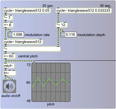
Once again we use all triangle functions, and we use a central pitch of 60 (middle C). The depth of pitch modulation -- plus or minus a certain number of semitones -- changes continuously, determined by the instantaneous value of a very-low-frequency oscillator with a peak amplitude of 12. Therefore, the depth will be as great as + or - 12 semitones, or as little as 0. The rate of the modulation varies from 1 Hz to 15 Hz, controlled by very-low-frequency oscillator that has a peak amplitude of 7 and an offset of 8 (so it varies up to + or - 7 Hz around its central rate of 8 Hz). Because these two control functions have different periodicities, the effect is continually changing, repeating exactly every 60 seconds.
In the next example we add one more modulator to continually change the central pitch, varying it up to + and - 30 semitones around a center of 66.
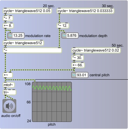
The central pitch will slowly, over the course of 50 seconds, rise from 66 to 96, fall to 36, then rise again to 66. The actual moment-to-moment pitch will oscillate up to 12 semitones around that, so the true pitch at any given instant could be as low as 24 or as high as 108, roughly the range of a piano. Since all three of these control functions have different periodicities -- 20, 30, and 50 seconds -- the entire cycle only repeats exactly every 5 minutes.
It's worth noting that as we combine different long cyclic phenomena with different periodicities -- in this case 20, 30, and 50 seconds -- the result of their combination varies continuously over a longer period that's equal to the product of the prime factors of the periods -- in this case 2 times 2 times 3 times 5 times 5 = 300 seconds. The effect is one of something that remains the same -- after all, it's the same three cycles repeating precisely over and over -- yet always seems slightly different because the juxtaposition and relationship of the cycles is always changing. This phenomenon is an essential component of much "minimal" or "phase" music.
In this first example we modulate both the rate and the depth (the frequency and the amplitude) of the LFO that is modulating the pitch of the carrier oscillator.
Once again we use all triangle functions, and we use a central pitch of 60 (middle C). The depth of pitch modulation -- plus or minus a certain number of semitones -- changes continuously, determined by the instantaneous value of a very-low-frequency oscillator with a peak amplitude of 12. Therefore, the depth will be as great as + or - 12 semitones, or as little as 0. The rate of the modulation varies from 1 Hz to 15 Hz, controlled by very-low-frequency oscillator that has a peak amplitude of 7 and an offset of 8 (so it varies up to + or - 7 Hz around its central rate of 8 Hz). Because these two control functions have different periodicities, the effect is continually changing, repeating exactly every 60 seconds.
In the next example we add one more modulator to continually change the central pitch, varying it up to + and - 30 semitones around a center of 66.
The central pitch will slowly, over the course of 50 seconds, rise from 66 to 96, fall to 36, then rise again to 66. The actual moment-to-moment pitch will oscillate up to 12 semitones around that, so the true pitch at any given instant could be as low as 24 or as high as 108, roughly the range of a piano. Since all three of these control functions have different periodicities -- 20, 30, and 50 seconds -- the entire cycle only repeats exactly every 5 minutes.
It's worth noting that as we combine different long cyclic phenomena with different periodicities -- in this case 20, 30, and 50 seconds -- the result of their combination varies continuously over a longer period that's equal to the product of the prime factors of the periods -- in this case 2 times 2 times 3 times 5 times 5 = 300 seconds. The effect is one of something that remains the same -- after all, it's the same three cycles repeating precisely over and over -- yet always seems slightly different because the juxtaposition and relationship of the cycles is always changing. This phenomenon is an essential component of much "minimal" or "phase" music.
Saturday, August 29, 2009
First steps in modulating the modulator
Classic waveforms can be used to shape music synthesis, and that idea can be extended to shape musical composition with simple, recognizable, repeating shapes. Indeed, many figures that we think of as traditional pitch patterns in pre-electronic music have a direct correlation with those classic waveforms. The picture below exemplifies simple melodic patterns in traditional notation that could be achieved with discrete sampling of classic waveforms at low frequency, used to control the pitch of a carrier sound.
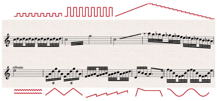
These melodic figures and their corresponding control functions can be described as:
1) trill, pulse wave
2) fingered tremolo, pulse wave with increased amplitude of modulation
3) glissando, linear ramp
4) scale, discrete sampling of a linear ramp
5) vibrato, triangle or sinusoid with low amplitude of modulation
6) up-down arpeggio, discrete sampling of a triangle function with high amplitude of modulation
7) melodic sequence, sawtooth (or any other shape) that is itself modulated by a ramp function
8) motivic melodic figure, discrete sampling of an arbitrary shape as it changes over time
9) up-down arpeggio (variation), discrete sampling of a sinusoidal function
You can probably imagine many other similar melodic shapes that are similarly simple yet effective.
These examples show clearly how a melody can be thought of as pitch modulation by a control function, and the shape can be simple, as in most of these examples, or more complex, as in example 8 above.
Sometimes more interesting effects can be achieved by using using these shapes operating at different formal levels at the same time, or with one shape modulating another as in example 7 above.
The triangle function, while decidedly not the most interesting shape imaginable, is particularly recognizable, and therefore is good for exemplifying these principles clearly. So we'll use it in a variety of examples for shaping sound synthesis and composition, focusing particularly on modulating one control function with a lower-frequency version of itself, which is to say, shaping the sound at a different formal levels, by means of self-similar use of a single shape.
The example below shows the most basic use of the triangle waveform as both a carrier oscillator and as a low-frequency control function for the pitch of that oscillator. The carrier oscillator generates a triangular waveform with the tri~ object which, instead of producing an ideal triangle function, protects against producing partials that will exceed the Nyquist frequency. The pitch of that oscillator is modulated by a low-frequency oscillator -- a cycle~ object reading from a wavetable that has been filled with one cycle of a triangle function. (When the patch is first opened, the small part of the program on the right fills the buffer~ with the values needed to make the stored triangle function. It also sets the scope~ to show one second of sound per display; the scope~ refreshes its display every 344 buffers of 128 samples.)
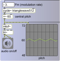
The modulating oscillator has a rate of 3 Hz, so the pitch of the carrier oscillator completes 3 cycles of the triangular shape per second. Since the amplitude of the cycle~ object is 1, the pitch fluctuates + and - 1 semitone around the central pitch of 60 (middle C). We'll call the rate of modulation Fm (pronounced "F sub m", meaning the frequency of the modulator), which is 3 Hz in this case, and we'll call the depth of modulation Am (pronounced "A sub m", meaning the amplitude of the modulator), which is constant at 1 in this case.
We can vary the pitch modulation over a longer period of time by modulating Fm and/or Am with an even slower oscillator. For example, in the program below we use one very-low-frequency oscillator to modulate the amplitude of a low-frequency oscillator that is modulating the pitch of the carrier oscillator.
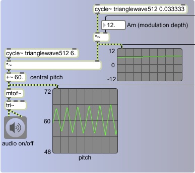 We have set Fm to a constant of 6 Hz, but Am is modulated by another oscillator with a rate of 1/30 Hz and an amplitude of 12. So every 30 seconds the depth of the "vibrato" changes, according to the triangle wave function, from 0 semitones to 12, to 0 to -12 and back to 0. You probably won't recognize the difference between a vibrato depth of + and - 12 semitones and its inverse, + or - -12 semitones, so in effect the vibrato seems to complete a full cycle of expansion and contraction once every 15 seconds.
So the pitch modulation, with a rate of 6 Hz, is itself modulated in amplitude repeatedly every 15 seconds. This is a simple case of a a modulator modulating a modulator.
These melodic figures and their corresponding control functions can be described as:
1) trill, pulse wave
2) fingered tremolo, pulse wave with increased amplitude of modulation
3) glissando, linear ramp
4) scale, discrete sampling of a linear ramp
5) vibrato, triangle or sinusoid with low amplitude of modulation
6) up-down arpeggio, discrete sampling of a triangle function with high amplitude of modulation
7) melodic sequence, sawtooth (or any other shape) that is itself modulated by a ramp function
8) motivic melodic figure, discrete sampling of an arbitrary shape as it changes over time
9) up-down arpeggio (variation), discrete sampling of a sinusoidal function
You can probably imagine many other similar melodic shapes that are similarly simple yet effective.
These examples show clearly how a melody can be thought of as pitch modulation by a control function, and the shape can be simple, as in most of these examples, or more complex, as in example 8 above.
Sometimes more interesting effects can be achieved by using using these shapes operating at different formal levels at the same time, or with one shape modulating another as in example 7 above.
The triangle function, while decidedly not the most interesting shape imaginable, is particularly recognizable, and therefore is good for exemplifying these principles clearly. So we'll use it in a variety of examples for shaping sound synthesis and composition, focusing particularly on modulating one control function with a lower-frequency version of itself, which is to say, shaping the sound at a different formal levels, by means of self-similar use of a single shape.
The example below shows the most basic use of the triangle waveform as both a carrier oscillator and as a low-frequency control function for the pitch of that oscillator. The carrier oscillator generates a triangular waveform with the tri~ object which, instead of producing an ideal triangle function, protects against producing partials that will exceed the Nyquist frequency. The pitch of that oscillator is modulated by a low-frequency oscillator -- a cycle~ object reading from a wavetable that has been filled with one cycle of a triangle function. (When the patch is first opened, the small part of the program on the right fills the buffer~ with the values needed to make the stored triangle function. It also sets the scope~ to show one second of sound per display; the scope~ refreshes its display every 344 buffers of 128 samples.)
The modulating oscillator has a rate of 3 Hz, so the pitch of the carrier oscillator completes 3 cycles of the triangular shape per second. Since the amplitude of the cycle~ object is 1, the pitch fluctuates + and - 1 semitone around the central pitch of 60 (middle C). We'll call the rate of modulation Fm (pronounced "F sub m", meaning the frequency of the modulator), which is 3 Hz in this case, and we'll call the depth of modulation Am (pronounced "A sub m", meaning the amplitude of the modulator), which is constant at 1 in this case.
We can vary the pitch modulation over a longer period of time by modulating Fm and/or Am with an even slower oscillator. For example, in the program below we use one very-low-frequency oscillator to modulate the amplitude of a low-frequency oscillator that is modulating the pitch of the carrier oscillator.
We have set Fm to a constant of 6 Hz, but Am is modulated by another oscillator with a rate of 1/30 Hz and an amplitude of 12. So every 30 seconds the depth of the "vibrato" changes, according to the triangle wave function, from 0 semitones to 12, to 0 to -12 and back to 0. You probably won't recognize the difference between a vibrato depth of + and - 12 semitones and its inverse, + or - -12 semitones, so in effect the vibrato seems to complete a full cycle of expansion and contraction once every 15 seconds.So the pitch modulation, with a rate of 6 Hz, is itself modulated in amplitude repeatedly every 15 seconds. This is a simple case of a a modulator modulating a modulator.
Sunday, August 2, 2009
Discrete steps within a continuous function
A series of discrete events can give the impression of a continuous progression. For example, the series of numbers 0, 2, 4, 6, 8, ... gives the impression of a straight linear progression, even though the series doesn't contain all the possible numbers along that line.
In fact, in digital media everything is a discrete step. Continuous phenomena are simulated by using a sufficiently high resolution of discrete steps. In digital video, for example, two-dimensional space is divided up into individual pixels, with each pixel having a color that is one of 16,777,216 discrete possibilities, time (the changing of the pixel values) is divided into 30 frames per second, and the audio stream is made up of 44,100 discrete amplitude values per second, with the instantaneous amplitude being one of 65,536 possible values.
A musical scale is another example of this. Like a ladder, a scale is a series of discrete steps in a linear progession. Even when the scale is not precisely linear, as in the case of a diatonic scale (steps 0, 2, 4, 5, 7, 9, 11, ... of the 12-tone chromatic scale), it still creates an impression of linear motion.
A smooth linear pitch glissando in computer music is achieved when the pitch value is changed continuously by a constant amount, usually as often as every single sample of the audio stream. If we employ the same control function but use it to change the frequency of the oscillator less frequently -- say, only a few times per second -- the pitch will stay steady for a longer time, and we'll perceive the discrete steps. Instead of changing the pitch 44,100 times per second, we could try using only 12 of those pitch values per second and holding the pitch steady in between.
This technique of transforming a high-resolution stream of numbers into a lower-resolution stream is known as "downsampling" -- reducing the rate or resolution of the discrete samples. In this case we want to reduce a stream of 44,100 samples per second to a series of only 12 samples per second. This process is achieved in audio with a technique called "sample and hold" -- in response to a triggering event, a single sample is held constant until the next trigger.
In Max, one way of doing this with an audio stream is with the sah~ object. A signal in the left inlet is sampled and held every time that the signal in the right inlet surpasses a particular threshold value.
This program uses sample and hold to turn a continuous pitch glissando function into a series of discrete scale steps.
The program is exactly like the example of using a triangle wave as a control function for a pitch glissando, except with a sah~ object inserted to convert the glissando into a scalewise series of discrete constant pitches. The cycle~ object going into the right inlet of sah~ has a frequency of 12 Hz, and it uses the triangle waveform stored in the buffer~ which increases past 0 at the beginning of each cycle. That triggers sah~ to sample and hold the current value of the pitch signal coming in the left intlet. So, whereas the pitch control oscillator is sending out a continuous glissando,
the sah~ object sends out a scalewise rendition of that shape by sampling and holding the pitch only once every 1/12 of a second.
The triangle shape is preserved, but the pitch is now in discrete steps of the chromatic scale at a rate of 12 notes per second instead of being a continuous glissando that changes pitch slightly with every sample. You can see that classic waveforms of electronic music synthesis can be applied in this way to serve as a control function even when the desired effect is individual notes of the tempered 12-tone scale.
Tuesday, June 23, 2009
Triangle wave as a control function
An object oscillating in simple harmonic motion, such as a pendulum swinging or a tuning fork vibrating, has a "restoring force" that pulls the object toward its central position -- gravity in the case of a pendulum, and tension in the case of a tuning fork. As the object approaches maximum displacement from the center it loses momentum due to the restoring force pulling against it. It loses velocity until its velocity is 0 and it then begins to be pulled in the opposite direction back toward the central position; it reaches maximum velocity in the center, overshoots the center due to its accrued momentum, and then increases its displacement in the opposite direction. This deceleration as it reaches maximum displacement, and acceleration as it is pulled away from maximum, is reflected in the smooth sinusoidal curve when we graph its displacement.
If there were no change in its velocity -- if it were to somehow instantaneously change direction with no deceleration and acceleration -- the graph of its displacement would look triangular.
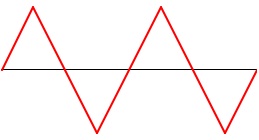
This sort of triangular function can be useful for representing constant periodic linear change -- back and forth, up and down, etc. -- between two extremes. In terms of sound, it's important to remember than the impression of linear change in the subjective phenomena of pitch and loudness actually correspond to exponential or logarithmic change in the empirical measures of frequency and amplitude.
If there were no change in its velocity -- if it were to somehow instantaneously change direction with no deceleration and acceleration -- the graph of its displacement would look triangular.
This sort of triangular function can be useful for representing constant periodic linear change -- back and forth, up and down, etc. -- between two extremes. In terms of sound, it's important to remember than the impression of linear change in the subjective phenomena of pitch and loudness actually correspond to exponential or logarithmic change in the empirical measures of frequency and amplitude.
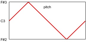
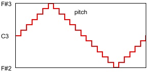
It's important to understand that a triangle function in pitch or decibels is not the same as a triangle function in frequency or linear amplitude. For example, a triangular displacement up and down from a central pitch by a tritone (+ or - 6 semitones) is exponential in frequency, and is a greater change upward in Hertz than it is downward. That is, a shift of 1/2 octave is a greater number of Hertz at higher frequencies than at lower frequencies, and a linear pitch change corresponds to an exponential curve in frequency, as illustrated in the following two visualizations. The first image depicts a linear change in pitch, as occurs in the program.
The second image depicts the change in frequency that corresponds to that triangle function in pitch.
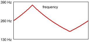 Note that the change in frequency is exponential rather than linear, and that a greater change of frequency is needed to go up a given pitch interval than is needed to go down the same pitch interval. In this case, to go from middle C (261.6 Hz) up to F# (370.0 Hz) is a difference of 108.4 Hz, while going down to F# (185.0 Hz) is a difference of 76.6 Hz. In Max the mtof or mtof~ object takes care of this translation from pitch to frequency for you. The formula in use is ƒ = 440.(2^(69.-p)), where p is the pitch in MIDI terminology (MIDI 69 = A 440 Hz).
A similar translation from linear to exponential is needed to go from the level in decibels, which is a logarithmic descriptor, to amplitude, which is on a linear scale. The formula used by the dbtoa and dbtoa~ objects to perform this translation is a = 10.^(d/20.), where d is the level in decibels relative to the maximum possible value, 1.
This program demonstrates the use of a triangular function to make periodic changes of pitch and loudness.
The second image depicts the change in frequency that corresponds to that triangle function in pitch.Note that the change in frequency is exponential rather than linear, and that a greater change of frequency is needed to go up a given pitch interval than is needed to go down the same pitch interval. In this case, to go from middle C (261.6 Hz) up to F# (370.0 Hz) is a difference of 108.4 Hz, while going down to F# (185.0 Hz) is a difference of 76.6 Hz. In Max the mtof or mtof~ object takes care of this translation from pitch to frequency for you. The formula in use is ƒ = 440.(2^(69.-p)), where p is the pitch in MIDI terminology (MIDI 69 = A 440 Hz).A similar translation from linear to exponential is needed to go from the level in decibels, which is a logarithmic descriptor, to amplitude, which is on a linear scale. The formula used by the dbtoa and dbtoa~ objects to perform this translation is a = 10.^(d/20.), where d is the level in decibels relative to the maximum possible value, 1.
This program demonstrates the use of a triangular function to make periodic changes of pitch and loudness.
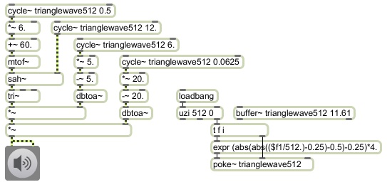
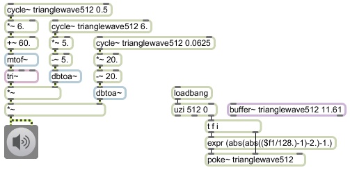
Instead of the cycle~ objects in this program reading from the default wavetable of 512 values in the form of a cosine function, we have to make a triangular function in a wavetable and read from that. The lower-right portion of the program creates and stores that function. When the program first starts up, it uses a mathematical expression to place 512 values in the form of a triangle wave into memory in a buffer~ object. (The size of the buffer -- 11.61 -- is expressed in milliseconds; at a sampling rate of 44,100 Hz, 11.61 milliseconds is 512 samples.)
The carrier oscillator is a tri~ object. Similarly to the saw~ and rect~ objects, tri~ generates a signal with a spectrum like that of a triangle wave, but one that limits its upper partials to avoid aliasing. This carrier oscillator's frequency and amplitude are controlled by three low-frequency oscillators -- the cycle~ objects reading from the triangle function in the buffer~. The triangle functions of the control oscillators are expressing values in terms of equal-tempered semitones and decibels, which correspond to our perception of pitch and volume, and those values are then converted to frequency and amplitude by the mtof~ and dbtoa~ objects.
Lets look at each of the uses of the triangle function here. At the top we have a triangle control oscillator with a frequency of 0.5 Hz, which means that it completes a cycle once every 2 seconds. Its amplitude is scaled by 6 and offset by 60, so it oscillates around the central value of 60, up as high as 66 and down as low as 54. This function is used to define the pitch, which is then translated into frequency by the mtof~ object and used to control the frequency of the carrier oscillator, the tri~ object. As in the other examples of classic control functions such as pulse wave, sawtooth wave, and sine wave, we use the triangle wave here as the carrier oscillator so that you can hear its timbral character. A triangle wave contains energy only at odd harmonics of the fundamental, with the amplitude of each partial proportional to the square of the inverse of the harmonic number. Thus, its timbre is richer than a sine tone, but mellower than a sawtooth wave.
The second triangle control oscillator has a frequency of 6 Hz, and serves to create an amplitude tremolo for the carrier oscillator. The control oscillates around -5 dB, going as high as 0 dB and as low as -10 dB. This level control is translated into amplitude by the dbtoa~ object and is used to control the amplitude of the carrier wave, creating a 10 dB fluctuation of amplitude 6 times per second.
The third triangle control oscillator has a frequency of 0.0625 Hz (1/16 Hz), so it completes a cycle only once every 16 seconds. This exerts a more formal function, creating a swell of the overall amplitude every 16 seconds, like a master volume knob, ranging as high as 0 dB and as low as -40 dB.
So in this one program we see the triangle function used 1) as a carrier waveform, for its timbral effect, with a frequency ranging from 185 to 370 Hz, 2) as a control function to create expressive amplitude tremolo at a rate of 6 Hz, 3) as a control function to create pitch glissando at a rate of 1/2 Hz, and 4) as a control function to create crescendo/decrescendo at a rate of 1/16 Hz.
Admittedly, the sound of an octave-wide pitch glissando is not terribly attractive; it's more like a siren than a musical gesture. But this program demonstrates several uses of this particular control function (timbre, glissando, tremolo, and dynamics), and shows the aesthetic effect of its characteristic shape.
Friday, June 19, 2009
Pulse wave, a binary control function
A pulse wave, also known as a rectangle wave, is a function that alternates periodically between two values, such as 1 and 0. This is a classic waveform of electronic music, and can be used as a control function to obtain an alternation between two states.
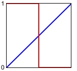


Max doesn't really provide a pulse wave generating object, but it's easy enough to create an ideal pulse wave by combining a phasor~ object, which ramps periodically from 0 to 1, and a <~ object, which will output only 1 or 0 depending on whether its input is less than a given value. For example, if you use <~ to test whether the value of the phasor~ is less than 0.5, the output will be 1 for the first half of the phasor~'s ramp, and 0 for the second half, resulting in a square wave.
We can then scale and offset the output of >~ to obtain a periodic alternation between any two desired values. In terms of musical pitch, a periodic alternation between two values is known as a trill or, in the case of a wider interval, a tremolo, and is usually at a fast but still sub-audio rate from about 8 to 18 notes per second. When the alternation takes place at an audio rate, the wave is heard as a pitched tone containing only odd harmonics, with the amplitude of each harmonic inversely proportional to the harmonic number. Thus, if the waveform has amplitude A, the fundamental (first harmonic) has amplitude A, the third harmonic has amplitude A/3, the fifth harmonic has amplitude A/5, etc. This means that upper harmonics may exceed the Nyquist frequency, possibly causing unwanted audible aliased frequencies. So for times when a rectangle waveform is desired for a carrier oscillator, there is an object called rect~ that generates a wave with a spectrum very similar to a rectangle wave, but that only produces audible harmonics up to the Nyquist frequency.
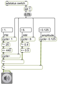
When a rectangle wave spends the same amount of time on 1 as it spends on 0, as in the above example, the wave is called a square wave. The amount of time the wave spends on 1, expressed as a fraction of one entire cycle, is called the duty cycle; in the case of a square wave the duty cycle is 0.5 because the wave spends 1/2 of its time at the value 1. However, a rectangle wave can have a duty cycle ranging anywhere from 0 to 1, which will allow a variety of alternation effects when the wave is used as a control function, and which will have a timbral effect when the wave is used as a carrier tone. For example, if we use 0.75 as the comparison value in the <~ object, the object's output will be 1 for 3/4 of each cycle of the phasor~, giving a rectangle wave with a duty cycle of 0.75.
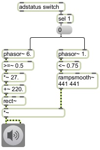
This program demonstrates the use of a pulse wave as a control function and as a carrier waveform, using modulator pulse wave LFOs to control both the frequency and the amplitude of the carrier wave.
In this example a square wave at a rate of 6 Hz is used to modulate the frequency of the carrier oscillator back and forth between 220 Hz and 247 Hz, which gives the impression of a musical trill between A 220 and the B above that, at the rate of 12 notes per second. In this case, rather than use a <~, we use a >=~ object so that the square wave will start with a 0 value, thus starting the trill on A 220. Note that for the carrier oscillator, the one we actually listen to, we have used the rect~ object, which gives a band-limited pulse tone that resists the aliasing effects of an ideal rectangle wave.
To control the amplitude in this example we use a rectangle wave with a rate of 1 Hz and a duty cycle of 0.75. The effect is that we hear the sound for 3/4 of a second, followed by 1/4 of a second of silence; we hear 9 notes of trill followed by three notes' worth of silence.
Because an instantaneous switch from an amplitude of 0 to an amplitude of 1 or vice versa would cause a click, we use the rampsmooth~ object to interpolate linearly to the new amplitude value over 441 samples (10 milliseconds).
Monday, June 15, 2009
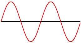
Sine wave as control function
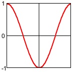
Sine and cosine are trigonometric functions that come from graphing the y or x value, respectively, of a point as it traverses the circumference of a unit circle in a constantly changing radial angle from 0 to 2π radians. The cosine is actually exactly the same as the sine with a phase offset of π/2 radians, which is to say starting 1/4 of a cycle into the sine function. To talk about any such function, regardless of phase offset, we can use the noun sinusoid and the adjective sinusoidal.
.jpg)
It happens that the sinusoid is also the graph of simple harmonic motion, such as the natural oscillation of a pendulum or the simple back-and-forth vibration of the tine of a tuning fork or an alternating electrical current. Simple harmonic motion is oscillation at a single frequency, so the sinusoidal wave is the most basic "building block" or elemental unit of all sound.
The cycle~ object in Max acts as a wavetable oscillator for generating periodic signals, and by default it uses the cosine function.
(Internally it is actually reading from a 512-point lookup table, and interpolating between those points as necessary to generate a smooth signal at any frequency.) Its peak amplitude is 1; it oscillates in the range from 1 to -1. Every time you turn on audio signal processing in Max, all cycle~ objects begin in cosine phase--i.e., starting at 1. However, you can supply a phase offset in the right inlet, so to make a cycle~ start with sine phase, you must supply a phase offset of 0.75 to start 3/4 of a cycle into the cosine function.
The sinusoidal oscillator can be used at an audio frequency as a carrier oscillator, or as a control function at a low frequency (or indeed any frequency) to modulate other signals. Since the sinusoidal oscillator was a basic generator in almost all early electronic synthesizers, we have become very familiar with the sound of using one oscillator for sinusoidal modulation of another oscillator's frequency and amplitude to create vibrato and tremolo effects. A singer or flutist will generally use a combination of vibrato and tremolo -- modulation of both frequency and amplitude of the tone -- for expressive effect at a rate somewhere between 5 to 8 Hz. Electronically and digitally, of course, we can modulate a tone at any rate, from extremely slow (such as 1/20 Hz) to audio rates (such as 2000 Hz). So we can use these different rates for sinusoidal control functions at the phrase level, the note level, or the microsonic timbral level.
This program demonstrates the use of the sine function for low-frequency modulation of a tone. One sine wave is the carrier oscillator that we actually hear, and the other three sine oscillators are the modulators.
When MSP is turned on, that fact is reported by the adstatus object, and that report is used to set the phase offset of the cycle~ objects to sine phase. This ensures that they all start with the correct, identical phase offset. The frequency is modulated + and - 25 Hz around a center frequency of 440 Hz. That's + and - about a semitone, so it fluctuates between approximately Bb and Ab around A 440. The amplitude is modulated + and - 0.4 around a center amplitude of 0.5. That's a total range from 0.9 to 0.1, which is a factor of 9, which is about 19 dB. Both of those ranges are larger than most singers or instrumentalists would ordinarily use for expressive vibrato, but they're made deliberately large here so they'll be obvious. The tremolo (amplitude modulation) rate is 6 Hz, which is about normal for idiomatic instrumental vibrato. However, the vibrato (frequency modulation) rate is only 1 Hz, which means it glides fairly slowly -- slowly enough that we can track its pitch -- and we tend to hear its extremes, Bb and Ab, as the main pitches. Interestingly, if you adjust the vibrato rate to be 6 Hz like the tremolo, the vibrato will be so fast that -- at this still fairly narrow pitch interval -- we tend to hear its center frequency, A 440, as the main pitch.
A third, very slow modulating sinusoid is used to shape the overall amplitude over a longer period of time. Its frequency is 1/8 Hz, which means that it completes one full cycle every 8 seconds. So, every 4 seconds it goes from 0 to peak amplitude (+ or -) and back to 0. Therefore, we hear a complete crescendo-diminuendo every 4 seconds. Even though the waveform is inverted when this modulator is negative, we don't perceive that fact when we listen to the tone in isolation, so amplification by a negative factor (the second half of the cycle of the modulating sinusoid) sounds the same to us as amplification by a positive factor (the first half of the cycle).
You can experiment with some different rates of modulation, including very slow and very fast (even audio rate) speeds.
Sunday, June 14, 2009
Classic waveforms as control functions
When using a computer to compose and play music, the distinction between music composition and sound synthesis becomes blurred. Since 1950 or so, composers' ways of conceiving musical sound and musical structure have been influenced by technological developments in electronic and computer sound synthesis and processing. This chapter and the next few chapters will provide some simple illustrations of how the electronic music technique of "modulation" -- using a waveform as a control function for another audio signal -- bears resemblance to some more traditional compositional techniques and structures. For simplicity and clarity, we'll start by using only classic electronic music waveforms: sine wave, rectangle wave, triangle wave, and sawtooth wave. We'll first show some sonic/musical effects of using those waveforms as modulators, then in subsequent chapters we'll increase the complexity by modulating the modulators, and then finally we'll make explicit the relationship between those classic sounds of electronic music and algorithmic composition with notes of the twelve-tone equal-tempered scale.
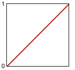
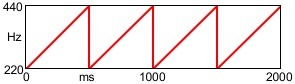 This example program uses a sawtooth function to make repeating frequency glissandi from 220 Hz to 440 Hz 2 times per second, using a phasor~.
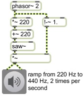 It uses the same phasor~ object to generate a simple amplitude envelope that goes immediately to 1 and ramps down to 0 at the same time as each glissando occurs.
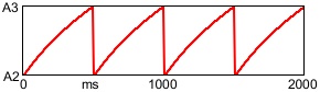
As shown in other chapters, a straight line function has many uses. When normalized as a ramp from 0 to 1, it's easy to enlarge it or contract it (with multiplication) and move it to a desired range (with addition) and even change its direction (by multiplying it by -1 or subtracting it from 1). The phasor~ object in Max provides a signal that ramps repeatedly from 0 to 1 at whatever frequency you specify.
This repeating ramp effectively creates a "sawtooth" function. By scaling it and offsetting it -- for example, by multiplying it by 220 and adding 220 to it -- we get a repeating ramp from 220 to 440 that can act as a control function for the frequency input of a carrier oscillator.
This example program uses a sawtooth function to make repeating frequency glissandi from 220 Hz to 440 Hz 2 times per second, using a phasor~.It uses the same phasor~ object to generate a simple amplitude envelope that goes immediately to 1 and ramps down to 0 at the same time as each glissando occurs.The carrier oscillator (the oscillator that generates the signal that we actually listen to) is also a sawtooth waveform. A sawtooth waveform produces a harmonic spectrum, with the amplitude of each harmonic inversely proportional to the harmonic number. Thus, if the waveform has amplitude A, the fundamental (first harmonic) has amplitude A, the second harmonic has amplitude A/ 2, the third harmonic has amplitude A/3, etc. This means that when the fundamental frequency is 440 Hz -- and when the audio sampling rate is 44,100 Hz -- harmonics above the 50th will be above the Nyquist frequency, yet will have an amplitude that is, in many cases, still audible. (The 51st harmonic will have an amplitude about 34 dB less than the fundamental.) Those upper partials will cause aliasing, so when a sawtooth waveform is desired for a carrier oscillator, an ideal sawtooth wave such as that generated by phasor~ is not always the best choice. In Max, there is an object called saw~ that generates a wave with a spectrum very similar to a sawtooth, but that only produces audible harmonics up to the Nyquist frequency. So for the carrier oscillator we use the band-limited sawtooth sound of saw~ rather than the ideal sawtooth wave of phasor~.
So in this simple example, we use a sawtooth waveform as the carrier signal, we modulate its frequency with a low-frequency sawtooth wave, and we use an inverted sawtooth wave at the same rate to generate amplitude envelopes that start loud and fade to 0. The result is repeating notes that glide up from 220 Hz to 440 Hz as the amplitude ramps from 1 to 0.
N.B. Because the glissandi are linear in frequency, they will actually be perceived as a logarithmic curve in terms of pitch.
Sunday, April 12, 2009
Control function as a recognizable shape
At the end of the article that defined a control function, I remarked that "One can think of a distinctive control function shape as being analogous to a musical motive or formal structure. The same motivic shape can occur over a long period of time (phrase level), or a short period (note level), or an extremely short period (for timbral effect)."
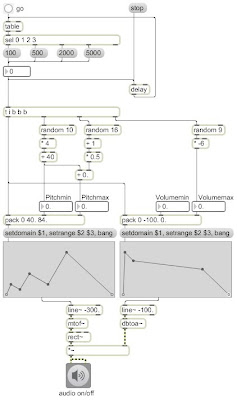
The shapes stay the same, but their transformations are chosen pseudo-randomly within specific ranges. The durations, which are also used as the delay time before starting the next shape, are chosen from among four possibilities: 100 ms, 500 ms, 2 sec, or 5 sec. The first duration will cause very short notes in which the envelope functions just have a timbral effect. The second duration is also a short note length (1/2 sec), but is just enough time for us to make out the shape within the note. The next two durations are definitely long enough for us to track the shape of the control functions as they affect pitch glissando and volume over the duration of a short "phrase".
The idea is that when a control function has a shape that is in some way distinctive and memorable, and that shape is used to control one or more parameters of a sound, the shape is exemplified by the sound, and the resulting sound will be recognizable when it recurs. In this way, it can function like a musical motive. And like a musical motive, it can remain recognizable as related to its original occurrence even if it undergoes certain modifications or transformations. Some typical types of transformations of a musical motive are rhythmic augmentation or diminution (multiplying the duration by a given amount to increase or decrease its total duration, and thus decrease or increase its speed), intervallic augmentation or diminution (keeping the contour the same but changing the size of its vertical range), transposition (moving it vertically by adding a certain amount to it), or delay (this is implicit in anything that recurs, because music takes place in time; delay is crucial to musical ideas such as imitation, canon, etc.). All of these can be crudely emulated mathematically with the simple operations of multiplication (to change the size of the shape horizontally and/or vertically) and addition (to offset the shape vertically or in time). Even as a motive is distorted by these manipulations, it retains aspects of its original shape, and its relationship to its original state can remain recognizable, serving an aesthetically unifying role.
Using the same shapes as were used in the example on line segment control functions, let's see how the shape of a control function can be distorted horizontally and vertically with multiplication and addition (i.e., by changing its range, transposition, duration, and delay). These multiple versions of the same shape can be assembled algorithmically into a musical passage. We'll use the same shapes as control functions, and apply them in the same way as before, to the pitch and amplitude of a simple synthesized tone. This program shows one way to compose and synthesize a sequence of related sounds using variations of a single control function.

The shapes stay the same, but their transformations are chosen pseudo-randomly within specific ranges. The durations, which are also used as the delay time before starting the next shape, are chosen from among four possibilities: 100 ms, 500 ms, 2 sec, or 5 sec. The first duration will cause very short notes in which the envelope functions just have a timbral effect. The second duration is also a short note length (1/2 sec), but is just enough time for us to make out the shape within the note. The next two durations are definitely long enough for us to track the shape of the control functions as they affect pitch glissando and volume over the duration of a short "phrase".
The durations are chosen using a distribution of probabilities. An important thing to notice about probabilistic choices of durations is that long durations take up much more time than short durations. So if we used an equal distribution of probabilities, the long notes would take up way more of the total time than the short notes, and it would give the effect of the long notes predominating. The proportion of the given durations is 1:5:20:50, so if each duration were chosen with equal likelihood, the 2-second and 5-second notes would take up 70/76 (92.1%) of the total time. To counter that effect, we can use a distribution that is the inverse of the proportions of the note durations. (See inside the table object.)
As in the earlier cited example, we use function objects to draw the function shapes, for each note we set the range and domain to the desired values, and then we bang the functions to cause them to send their information to the line~ objects.
It's important to note that in this example, instead of the line segment functions controlling frequency and amplitude of the synthesized sound directly, they control the subjective parameters pitch and volume, specified as MIDI note names and decibels, respectively. Much has been written on the logarithmic nature of subjective perception relative to empirical measurement. This is particularly demonstrable in the case of musical pitch and loudness. We perceive these subjective traits as the logarithm of the empirical sonic attributes called fundamental frequency and amplitude. Fortunately, that logarithmic relationship makes it fairly easy to do a mathematical translation from a linear pitch difference or loudness difference into the appropriate exponential curve in the physical attribute of frequency or amplitude. The formula for translating MIDI pitch m into frequency f, according to the 12-notes-per-octave equal-tempered tuning system is f=440(2^((69-m)/12)). Using the reference frequency of A=440 Hz, which is equivalent to MIDI note number 69, multiply that times the (69-m)/12th root of 2. Max provides objects called mtof (for individual Max messages) and mtof~ (for signals) that do this math for you. The formula for translating volume in decibels d into amplitude a is a=10^(d/20). The amplitude a is calculated as 10 to the power of (d/20). This makes a reference of 0 dB equal to an amplitude of 1 (the greatest possible amplitude playable by Max signal processing), and all negative decibel values will result in an amplitude between 1 and 0. Max provides objects called dbtoa and dbtoa~ to do this math for you.
The arguments in the line~ objects might look a little strange, and they're not very important; they were chosen just to keep the program from making any sound when it's first opened. There's not really a MIDI pitch number that corresponds to a frequency of 0 (which would stop the rect~ oscillator)--MIDI pitch number 0 is a super-low C that would actually have a fundamental frequency of 8.1758 Hz--but -300 is a hypothetical MIDI number that would slow the oscillator down to about 0 Hz. Similarly, there is no decibel value that would truly give an amplitude of 0 (it would have to be negative infinity!), but -100 dB is equal to an amplitude of 0.00001, which is for all practical purposes inaudible.
Now let's look at the actual numbers being used for the pitches and volumes. The volume (peak amplitude) of each note will be one of nine possible decibel values, ranging from 0 dB (fff) to -48 dB (ppp) in increments of 6 dB. That's a pretty wide dynamic range for the peak amplitudes; it's at least as wide as most instrumentalists habitually use. Of course, recording systems need a much wider range than this to record all the subtleties of sounds in their quietest moments, but I'm just referring to the dynamic range of the peak amplitudes (the attacks) of the notes. The low end of the pitch range for each note will be one of 10 possible pitches, ranging from E just below the bass staff (MIDI 40) to E at the top of the treble staff (MIDI 76), in increments of a major third (4 semitones). The size of the range (the difference between Pitchmin and Pitchmax) will range from 0.5 to 8 semitones (from 1/4 tone to a minor 6th), as measured in 16 quarter-tone steps. This gives a possibility of some relatively wide glissandi and some very subtle small ones.
To test this program, just start the audio and click on the go button. Notice that most of the notes are very short (100 ms or 500 ms), with occasional longer notes (2 sec or 5 sec). The dynamics are arbitrarily and equally distributed from ppp to fff, and the pitches are arbitrarily and equally distributed from low to high, with a variety of glissando ranges.
My contention is that even though the compositional decisions made by the computer are arbitrary and undistinguished in their own right, there is a sense of unity and consistency to the sounds being played, due to the constant use of single shapes for pitch glissando and amplitude envelope, and that this helps to give an impression of coherency and intentionality. That is presumably the main utility of motive in composition: it gives a sense of repetition, recognizable variation, and consistency to a variety of different sounds.
Wednesday, April 1, 2009
Line-segment control function
In the article on fading by linear interpolation, you can see a demonstration of how a particular characteristic of a sound or an image (such as the amplitude of a sound or the brightness of an image) can be modified gradually over time. A word that's important for this type of operation is parameter, which means a numerical descriptor of a characteristic. For example, amplitude and brightness can each be controlled by a single number representing "gain" (the factor by which we turn it up or down). In that example using a "gain" factor to control amplitude or brightness simply involves multiplying the signal (the thing you want to modify) by the gain factor. In the case of audio, we multiply every single individual sample of the audio signal (tens of thousands of samples per second) by the gain factor; in the case of video we multiply every color value of every pixel of every frame by the gain factor. (That is exactly what the "brightness" operation is doing internally in the jit.brcosa object.) In each case, a single number sets a precise amount by which we modify a particular parameter. When discussing a sound or an image or a musical passage or a video, there are often many characteristics that can be usefully described by a number. When you get right down to it, it's usually possible to convert nearly any description into one or more numbers somehow, and once you've done that, the description can then be manipulated by arithmetic operations.
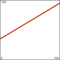
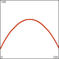
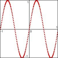
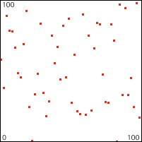
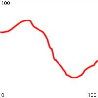
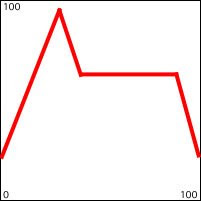
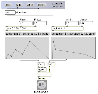 For the amplitude function, a shape has been chosen that is similar to the amplitude envelope of many instruments when the function takes place over a duration of about 500 to 2000 milliseconds. For the frequency function, a shape has been chosen that results in three up-down glissandi that increase in range and duration. Try listening to these control functions at different durations. When played very slowly over 10 seconds, the envelopes are clearly audible as gradual frequency glissandi and amplitude changes. When played over a quicker duration such as 1/2 second, the amplitude envelope sounds quite natural and the glissandi are quick and almost melodic. When played extremely fast, over 1/10 of a second, the glissandi are too fast to perceive as such, and the effect is mostly timbral. Try also changing the frequency range values to see what effect occurs when the range is very small or very large.
So, as we saw in that example, when a parameter changes over time, it can create an interesting change in aesthetic effect (such as a fade in or out). The change in that case was linear and directional. That makes for a simple yet clear and direct type of change. You can think of the straight line as one simple kind of shape imposed on the characteristic being controlled. Other shapes such as smooth curves or irregular patterns are also possible.
Before we go on, let's define a couple of words: the nouns control and function.
A control is something that we don't perceive directly, but the effect of which we can perceive when it's applied to a parameter. For instance, in the fading by means of linear interpolation example, we don't literally see a line or hear a line, but we perceive the linear effect when the line is applied to the gain factor that controls brightness and amplitude.
A function is a defined relationship between two variables. Let's call those variables x and y, which could stand for anything. In general one variable, x, stands for something "given" or "known" (an example might be time, which we can know with some accuracy using a clock), and the other variable, y, stands for something the value of which will depend upon the value of x. We say that "y varies as a function of x", which means that there is a known relationship that permits us to know the value of y if we know the value of x. Often the relationship between x and y can be perfectly described by a mathematical equation that contains two variables, x and y. That's what mathematicians generally mean when they use the word function: an equation that permits you to calculate the value of y for every possible value of x you might put into the equation. That's what's being described by the examples in the article on the mathematical manipulation of digital media. The formulae such as y=x, or y = Asin(2πƒt+ø)+d, or y=mx+b are examples of functions in which the value of y depends on the value of x in a way that can be reliably calculated. If we plug many different values of x into the equation and calculate y for each one, and graph the results with x on the horizontal axis and y on the vertical axis, we'll get a shape. That shape is called the "graph of the function". But a mathematical equation is not the only way to define a relationship between two variables.
A function could also be a shape that is not easily described by a mathematical equation, and we would discover the value of y by mapping it to its corresponding x value on the graph. Another way would be to actually have a listed series of all possible x values and the y values that correspond with them. These methods may take a bit more memory to store a complex shape or a list of x,y pairs, but a) they allow us to use shapes that are not easily described mathematically and b) rather than requiring calculation, they just require a quick lookup of the y value based on the known x value.
But regardless of the precise method of establishing the relationship between the known variable and the unknown variable--whether it's done by a calculation or a lookup--one important characteristic of a function is that it describes a knowable one-to-one relationship (of any degree of complexity) between x values and y values.
So, by combining those two words, we arrive at an expression that is used frequently in audio sound synthesis, and which, as we will see, can also be used in algorithmic composition: control function. A control function is a shape that is used to control a parameter in sound or music or video or animation. Most commonly x is the passage of time, and y is the value of some parameter over that period of time. All kinds of shapes are potentially useful as control functions.
Straight lines

Curves

Trigonometric functions

Random or arbitrary x,y pairs

Freehand drawn shapes

Combinations of line segments

We'll look at how some of these control functions can be used to control or modify sounds, and then we'll transfer some of that thinking into the control of attributes of a musical structure or an animation. We'll start with line segment shapes such as the one depicted directly above.
The article on linear change introduces some of the math involved in making a formulaic description of linear change over time, and the article on linear interpolation introduces the handy Max object called line. The line object lets you just specify a destination value (the value you want to get to), a transition time (how long you want to take to get there), and a reporting interval (how often you want it to send out intermediate values along the way there), and it sends out a timed series of values that progress linearly from its current value to the destination value in the specified amount of time. Max also provides a line~ object for doing the same thing for an audio signal. The messages you send to a line~ object differ from those of line in two significant ways. First of all, there is no argument for the "reporting interval" in line~ because line~ sends out an audio signal, and every single sample of that signal reports an intermediate value interpolated between the starting value and the destination value; in effect, the reporting rate is the same as the audio sampling rate. So all line~ really requires is two numbers: the destination value and the transition time. The other difference is that line~ can receive multiple value-time pairs in the same message, all as part of the same list. For example, a message such as '1. 1500 0.5 500 0.5 2000 0. 6000' will cause line~ to send out a signal that goes to 1 in 1500 milliseconds, goes from 1 to 0.5 in 500 milliseconds, stays at 0.5 for 2000 milliseconds, goes to 0 in 6000 milliseconds, and stays at 0 until it receives a message causing it to go to a different value. In this way a single message can describe a function over time made up of several straight line segments.
The function object allows the user to draw a line-segment shape of this sort. When the object receives a 'bang' it sends out such a message (intended for line~) that will cause line~ to send out that function shape. The minimum and maximum of the range (of the y axis) of the function can be set by a 'setrange' message, and the duration (of the x axis) can be set by a 'setdomain' message.
This patch shows the use of line segment control functions to shape the frequency and amplitude of a tone. When you choose a duration for the function, that number is used to set the domain of the function objects (and also uses whatever values have been chosen for the minimum and maximum of the frequency and amplitude ranges).
 For the amplitude function, a shape has been chosen that is similar to the amplitude envelope of many instruments when the function takes place over a duration of about 500 to 2000 milliseconds. For the frequency function, a shape has been chosen that results in three up-down glissandi that increase in range and duration. Try listening to these control functions at different durations. When played very slowly over 10 seconds, the envelopes are clearly audible as gradual frequency glissandi and amplitude changes. When played over a quicker duration such as 1/2 second, the amplitude envelope sounds quite natural and the glissandi are quick and almost melodic. When played extremely fast, over 1/10 of a second, the glissandi are too fast to perceive as such, and the effect is mostly timbral. Try also changing the frequency range values to see what effect occurs when the range is very small or very large.
The point here is that the same functions can be "stretched" (augmented or diminished) over a variety of durations and/or ranges to create a wide variety of sonic/musical effects without changing the basic shape of the control functions. One can thus think of a distinctive control function shape as being analogous to a musical motive or formal structure. The same motivic shape can occur over a long period of time (phrase level), or a short period (note level), or an extremely short period (for timbral effect). In this program, one can also simply draw a new control function with the mouse, to create a new motive.
Subscribe to:
Posts (Atom)