Line-segment control function

In the article on fading by linear interpolation, you can see a demonstration of how a particular characteristic of a sound or an image (such as the amplitude of a sound or the brightness of an image) can be modified gradually over time. A word that's important for this type of operation is parameter, which means a numerical descriptor of a characteristic. For example, amplitude and brightness can each be controlled by a single number representing "gain" (the factor by which we turn it up or down). In that example using a "gain" factor to control amplitude or brightness simply involves multiplying the signal (the thing you want to modify) by the gain factor. In the case of audio, we multiply every single individual sample of the audio signal (tens of thousands of samples per second) by the gain factor; in the case of video we multiply every color value of every pixel of every frame by the gain factor. (That is exactly what the "brightness" operation is doing internally in the jit.brcosa object.) In each case, a single number sets a precise amount by which we modify a particular parameter. When discussing a sound or an image or a musical passage or a video, there are often many characteristics that can be usefully described by a number. When you get right down to it, it's usually possible to convert nearly any description into one or more numbers somehow, and once you've done that, the description can then be manipulated by arithmetic operations.

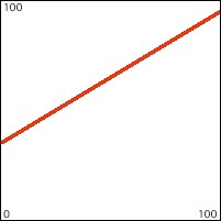
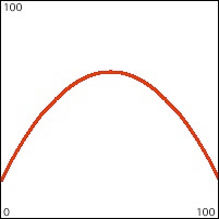
So, as we saw in that example, when a parameter changes over time, it can create an interesting change in aesthetic effect (such as a fade in or out). The change in that case was linear and directional. That makes for a simple yet clear and direct type of change. You can think of the straight line as one simple kind of shape imposed on the characteristic being controlled. Other shapes such as smooth curves or irregular patterns are also possible.

Before we go on, let's define a couple of words: the nouns control and function.

A control is something that we don't perceive directly, but the effect of which we can perceive when it's applied to a parameter. For instance, in the fading by means of linear interpolation example, we don't literally see a line or hear a line, but we perceive the linear effect when the line is applied to the gain factor that controls brightness and amplitude.

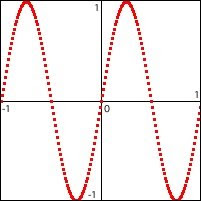
A function is a defined relationship between two variables. Let's call those variables x and y, which could stand for anything. In general one variable, x, stands for something "given" or "known" (an example might be time, which we can know with some accuracy using a clock), and the other variable, y, stands for something the value of which will depend upon the value of x. We say that "y varies as a function of x", which means that there is a known relationship that permits us to know the value of y if we know the value of x. Often the relationship between x and y can be perfectly described by a mathematical equation that contains two variables, x and y. That's what mathematicians generally mean when they use the word function: an equation that permits you to calculate the value of y for every possible value of x you might put into the equation. That's what's being described by the examples in the article on the mathematical manipulation of digital media. The formulae such as y=x, or y = Asin(2πƒt+ø)+d, or y=mx+b are examples of functions in which the value of y depends on the value of x in a way that can be reliably calculated. If we plug many different values of x into the equation and calculate y for each one, and graph the results with x on the horizontal axis and y on the vertical axis, we'll get a shape. That shape is called the "graph of the function". But a mathematical equation is not the only way to define a relationship between two variables.

A function could also be a shape that is not easily described by a mathematical equation, and we would discover the value of y by mapping it to its corresponding x value on the graph. Another way would be to actually have a listed series of all possible x values and the y values that correspond with them. These methods may take a bit more memory to store a complex shape or a list of x,y pairs, but a) they allow us to use shapes that are not easily described mathematically and b) rather than requiring calculation, they just require a quick lookup of the y value based on the known x value.

But regardless of the precise method of establishing the relationship between the known variable and the unknown variable--whether it's done by a calculation or a lookup--one important characteristic of a function is that it describes a knowable one-to-one relationship (of any degree of complexity) between x values and y values.

So, by combining those two words, we arrive at an expression that is used frequently in audio sound synthesis, and which, as we will see, can also be used in algorithmic composition: control function. A control function is a shape that is used to control a parameter in sound or music or video or animation. Most commonly x is the passage of time, and y is the value of some parameter over that period of time. All kinds of shapes are potentially useful as control functions.

Straight lines

Curves

Trigonometric functions

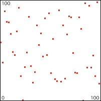
Random or arbitrary x,y pairs

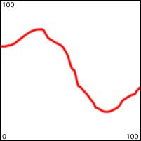
Freehand drawn shapes

Combinations of line segments

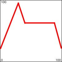
We'll look at how some of these control functions can be used to control or modify sounds, and then we'll transfer some of that thinking into the control of attributes of a musical structure or an animation. We'll start with line segment shapes such as the one depicted directly above.

The article on linear change introduces some of the math involved in making a formulaic description of linear change over time, and the article on linear interpolation introduces the handy Max object called line. The line object lets you just specify a destination value (the value you want to get to), a transition time (how long you want to take to get there), and a reporting interval (how often you want it to send out intermediate values along the way there), and it sends out a timed series of values that progress linearly from its current value to the destination value in the specified amount of time. Max also provides a line~ object for doing the same thing for an audio signal. The messages you send to a line~ object differ from those of line in two significant ways. First of all, there is no argument for the "reporting interval" in line~ because line~ sends out an audio signal, and every single sample of that signal reports an intermediate value interpolated between the starting value and the destination value; in effect, the reporting rate is the same as the audio sampling rate. So all line~ really requires is two numbers: the destination value and the transition time. The other difference is that line~ can receive multiple value-time pairs in the same message, all as part of the same list. For example, a message such as '1. 1500 0.5 500 0.5 2000 0. 6000' will cause line~ to send out a signal that goes to 1 in 1500 milliseconds, goes from 1 to 0.5 in 500 milliseconds, stays at 0.5 for 2000 milliseconds, goes to 0 in 6000 milliseconds, and stays at 0 until it receives a message causing it to go to a different value. In this way a single message can describe a function over time made up of several straight line segments.

The function object allows the user to draw a line-segment shape of this sort. When the object receives a 'bang' it sends out such a message (intended for line~) that will cause line~ to send out that function shape. The minimum and maximum of the range (of the y axis) of the function can be set by a 'setrange' message, and the duration (of the x axis) can be set by a 'setdomain' message.

This patch shows the use of line segment control functions to shape the frequency and amplitude of a tone. When you choose a duration for the function, that number is used to set the domain of the function objects (and also uses whatever values have been chosen for the minimum and maximum of the frequency and amplitude ranges).

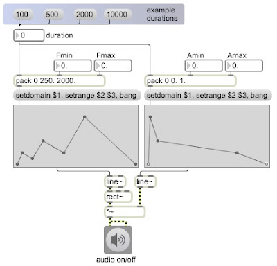For the amplitude function, a shape has been chosen that is similar to the amplitude envelope of many instruments when the function takes place over a duration of about 500 to 2000 milliseconds. For the frequency function, a shape has been chosen that results in three up-down glissandi that increase in range and duration. Try listening to these control functions at different durations. When played very slowly over 10 seconds, the envelopes are clearly audible as gradual frequency glissandi and amplitude changes. When played over a quicker duration such as 1/2 second, the amplitude envelope sounds quite natural and the glissandi are quick and almost melodic. When played extremely fast, over 1/10 of a second, the glissandi are too fast to perceive as such, and the effect is mostly timbral. Try also changing the frequency range values to see what effect occurs when the range is very small or very large.

The point here is that the same functions can be "stretched" (augmented or diminished) over a variety of durations and/or ranges to create a wide variety of sonic/musical effects without changing the basic shape of the control functions. One can thus think of a distinctive control function shape as being analogous to a musical motive or formal structure. The same motivic shape can occur over a long period of time (phrase level), or a short period (note level), or an extremely short period (for timbral effect). In this program, one can also simply draw a new control function with the mouse, to create a new motive.