Monday, September 29, 2008

A simple probabilistic decision

In all of the examples of autonomous computer decision making presented up to this point, we've used equal probabilities for all the possible choices, using the random object or its audio counterpart noise~. The resultant choices have thus been truly arbitrary, within the limits prescribed by the program.

It's also possible to use random number generation to enact decisions that are still arbitrary but are somewhat more predictable than plain randomness. One can apply a probability factor to make one choice more likely than another in a binary decision, or (as will be demonstrated in a future lesson) one can apply a more complicated probability function to a set of possibilities, giving each one a different likelihood. This lesson will demonstrate the first case, using a probability factor to make a binary decision in which one result is more likely to occur than the other.

As described briefly in an earlier lesson on randomness, the probability of a particular looked-for event occurring can be defined as a number between 0 and 1 inclusive, with that number being the ratio of the number of looked-for outcomes divided by the number of all possible outcomes. For example, the probability of choosing the the ace of spades (1 unique looked-for result) out of all possible cards in a deck (52 of them) is 1/52, which is 0.019231. The probability of not choosing the ace of spades is 1 minus that, which is 0.980769 (51/52). Thus we can say that the likelihood of choosing the ace of spades at random from a deck of cards is less than 2%, and the likelihood of not choosing it is a bit more than 98%; other ways of stating this are to say that there is a 1 in 52 chance of getting the ace of spades, or to say that the odds against choosing the ace of spades are 51 to 1.

For making an automated decision between two things, we can emulate this sort of odds by applying a probability factor between 0 and 1 to one of the choices. For example, if we want to make a decision between A and B, with both being equally likely, we would set the probability of A to 0.5 (and thus the probability of B would implicitly be 1 minus 0.5, which also equals 0.5). If we want to make A somewhat more likely than B, we could set the probability of A to something greater than 0.5, such as 0.75. This would mean there is a 75% chance of choosing A, and a 25% chance of choosing B; the odds in favor of choosing A are 3 to 1 (75:25). This does not ensure that A will always be chosen exactly thrice as many times as B. It does mean, however, that as the number of choices increases, statistically the percentage of A choices will tend toward being three times that of B.

The simplest way to do this in a computer program is as follows: Set the probability P for choice A. Choose a random number x between 0 and 1 (more specifically, 0 to just less than 1). If x is less than P, then choose A; otherwise, choose B. The result of such a program will be that over the course of numerous choices, the distribution of A choices over the total number of choices will tend toward P. The choices will still be arbitrary, and we can't predict any individual choice with certainty (unless the probability of A is either 0 or 1), but we can characterize the statistical probability of choosing A or B.

Because the random generator in Max produces whole numbers less than the specified maximum rather than fractional numbers between 0 and 1, we have to do one additional step: we either have to map the range of random numbers into the fractional 0-to-1 range, or we have to map the probability factor into the range of whole numbers. It turns out to be slightly more efficient to do the latter, because it requires doing just one multiplication when we specify the probability, rather than doing a division every time we generate a random number. The following tiny program does just that. Every time it receives a message in its inlet, it will make a probabilistic choice between two possible results, based on a provided probability factor.
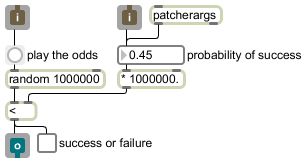
The probability value that goes into the number box (either by entering the number directly or by it coming from the right inlet or the patcherargs obejct) gets multiplied by 1,000,000 and the result is stored in the right inlet of the less than object. The bang from the button (triggered either by a mouse click or by a message coming in the left inlet) causes random to generate a random number from 0 to 999,999. If it is less than the number that came from the probability factor (which would be 450,000 in the above example), it sends out a 1, otherwise it sends out a 0. You can see that statistically, over the course of many repetitions, it will tend to send out 1 about 45% of the time.

A useful programming trick that is invisible in this picture is that the number box has been set to have a minimum value of 0 and a maximum value of 1. Any value that comes in its inlet will be clipped to that range before being sent out, so the number box actually serves to limit the range and prevent any inappropriate probability values that might cause the program to malfunction. Protecting against expected or unwanted values, either from a user or from another part of the program, is good safe programming practice.

As was mentioned earlier, the multiplication of the probability by 1,000,000 is because we want to express the probability as a fraction from 0 to 1, but random only generates random whole numbers, so we need to reconcile those two ranges. We chose the number 1,000,000 because that means that we can express the probability to as many as six decimal places, and when we multiply it by 1,000,000 the result will always be a unique integer representing one of those 1,000,001 possible values (from 0.000000 to 1.000000 inclusive). Since six decimal places is the greatest precision that can be entered into a standard Max object, this program takes full advantage of the precision available in Max. It's inconceivable that you could create a situation in which you could ever hear the difference between a 0.749999 probability and a 0.750000 probability (indeed, in most musical situations it's doubtful you could even hear the difference between a 0.74 probability and a 0.75 probability), but there's no reason not to take advantage of that available precision.

Notice that this little program has been written in such a way that it can be tried out with the user interface objects number box, button, and toggle, but it was actually designed to be useful as a subpatch in some other patch, thanks to the inclusion of the inlet, outlet, and patcherargs objects. All of its input and output is actually expected to come from and go to someplace else in the parent patch, for use in a larger program. The number box clips any probability value to the 0-to-1 range, and the button converts any message in the left inlet to a bang for random. Save this patch with the name gamble, because it is used in the next example patch.

Now that we have a program that reliably makes a probabilistic decision, we'll use it to make a simple binary decision whether to play a note or not.

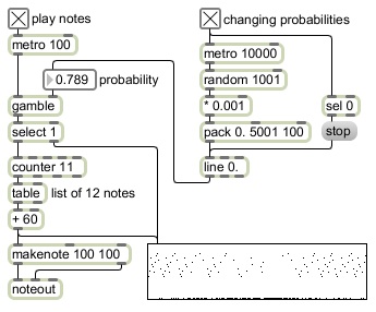
If the metro 100 object were connected directly to the counter 11 object, the patch would repeatedly count from 0 to 11, to cycle through a list of twelve pitch classes stored in the table, to play a loop at the rate of ten notes per second. However, as it is, the metro 100 object triggers the gamble object to make a probabilistic decision, 1 or 0. The select 1 object triggers a note only if the choice made by gamble is 1. If you click on the toggle to turn on the metro 100 object you will initially hear nothing because the probability of gamble choosing a 1 is set to 0. If you change the probability value to 1., gamble will always choose 1, and you will hear all the notes being played.
If the probability is set to some value in between 0 and 1, say 0.8, gamble will, on average, choose to play a note 80% of the time and choose to rest 20% of the time. The exact rhythm is unpredictable, but the average density of notes per second will be 8.

The upper right part of the patch randomly chooses a new probability somewhere in the range from 0 to 1 every ten seconds, and uses linear interpolation to arrive at the newly chosen probability value in five seconds. The probability will then stay at that new value for five seconds before the next value is chosen. By turning on this control portion of the patch, you can hear the effect of different statistical note densities in time, and the gradual transition from one density to another over five seconds.

Note that when gamble chooses 0, no note is played but the select 1 object still sends the 0 to the multislider (but not to the counter) so that the musical rest is shown in the graphic display, creating the proper depiction of the note density.

In this lesson we made a useful subpatch for making probabilistic decisions, and we used those decisions to choose whether to play a note or not. Of course the decision could be between any two things. For example you might use it to make control decisions, at a slower rate, choosing whether to run one part of the program or another, to control a longer-term formal structure.

Sunday, September 28, 2008

Moving range of random choices

The previous example used a very slow metronome to cause a change in the music every five seconds -- specifically to choose a new range of random pitch numbers for the note-playing algorithm. Because the change happens suddenly at a specific moment in time, the change in the musical texture is abrupt, creating a distinct new block of notes every five seconds.

Just as we used linear interpolation in earlier chapters to play a scale from one pitch to another or to create a fade-in of loudness or brightness, we could also use linear interpolation to cause more gradual change in the range of random numbers being used in a decision making process. Instead of changing the range and offset of the random numbers abruptly, we could just as well interpolate from the current range settings to the new range settings over a period of time.

This patch is in some ways very similar to the previous one, but the big difference here is the introduction of the line object to make a gradual transition to a new range of random numbers over time.
Instead of the new ranges going directly to the right inlet of the + object and the random object, they go to line objects, which send out a changing series of numbers that move to the new value over the course of five seconds. The pack objects are there to make well-formed messages for the line objects, telling line what transition time to use (5000 ms) and how often to send out an intermediate number (every 125 ms).

As in the previous example, the random 88 object chooses the offset from the bottom of the piano keyboard, which will have 21 added to it and be used as the minimum value for the random range. That same number also is subtracted from 88 to set the maximum possible size of the randomly chosen pitch range, so as not to exceed the total range of the piano; the range size that actually gets chosen is thus some random number up to that maximum.

This patch also differs from the previous one in that it varies the MIDI velocities of the notes as well as the pitches, to create some dynamic variation of loudness. To do this, the program chooses one of only six possible ranges (with the random 6 object), which one might think of as being analogous to the musical dynamic markings pp, p, mp, mf, f, and ff. Those random numbers 0 to 5 are multiplied by 20 and added to 8, so that the possible offsets for the velocity range are 8, 28, 48, 68, 88, and 108. The size of the velocity range is always 20 (as determinied by the random 20 object) so there will always be the same range of variety in the velocities, but the range itself will almost always be moving continuously up or down because of the changing offset.

The transition time of 5000 ms for all of the line objects performing the gradual range changes was chosen to be the same as the interval of the metro object that is triggering the changes. However, the transition time could in fact be chosen to be quicker, all the way down to 0 ms for an immediate change. The interval of change choices by the metro and the transition time for the line objects have been set equal in this example so that the changes are constant and completely gradual, but in fact the two things could be treated as independent (that is, changes could be sometimes sudden and other times gradual).

There are still many more ways in which the musical form and texture could be varied in this sort of simple random decision making algorithm. For example, the rate of the note-playing metro could be varied continuously in a manner similar to the way pitch and velocity are being varied here, which would cause acceleration and deceleration of the note rate. It would also be possible to randomly change the time interval of the choice-making metro in order to to vary the frequency with which new choices are made. Also, currently all note durations are the same as the inter-onset interval between notes; one can thus say that the ratio of duration to IOI is 1. However, an algorithm could include random variation of that ratio describing note duration as a factor of the inter-onset interval, to create either staccato notes (silence between notes) if the factor is less than 1, or overlapping notes if the factor is greater than 1. We'll see use of this legato factor in a future example. There could also be a part of the algorithm for making random decisions about presses of the piano's sustain pedal (MIDI controller number 64). Obviously musical composition usually involves much more than just decisions about pitch and loudness.

This example and the previous one have shown how changes in the range of possibilities can create interesting variation even with simple random decisions, and that the changes can be either abrupt or gradual for different effects. These principles of controlling the size and offset of crucial ranges are useful even when dealing with non-random decision making.

Sunday, September 14, 2008

Limiting the range of random choices

The previous examples showed random selection from a body of possible choices. In the first example of randomness the selection was from among events that had a certain distinctive character (chords, paintings, drum sounds), such that the events were fairly engaging in their own right and the order in which they occurred was not terribly crucial. In the next example, showing the relationship of randomness and noise, the individual events were neutral and and relatively characterless (individual samples in an audio signal, or pitches in a steady stream of notes), so the result was maximally patternless and colorless because all possibilities could occur with equal likelihood. In the case of random audio samples we get white noise (confirming the description as "colorless"), and in the case of random pitches we get complete atonality.

Even with such random decision making, however, we can still exert some control to shape the random selections in various ways. One way is simply to limit ourselves to a subset of the full range of possibilities. The subset will in some way be distinct from the full set, and that will allow us to characterize it by the way(s) in which it differs from the full set. For example, instead of choosing randomly from among all the keys of the piano--MIDI notes 21 to 108 as in the previous example-- we could decide to choose from a smaller number of notes. If the subset we choose is significantly different from the full set, we'll recognize the difference. (In effect, we'll recognize the absence of certain possibilties.) For example, if we choose only from among the pitches 59 to 70, we could characterize those pitches as "middle range" because we would observe that the choices contained no very low or very high notes. Choices made in this way would be noticeably different from choices made in the range 21 to 32 (extremely low), or 97 to 108 (extremely high), or 95 to 96 (very high and extremely small range), or 21 to 66 (low but very wide range), and so on. In this way we can get variety and distinction between different subsets of possible choices, even though the decision making method within the specified range would still be completely random.

This example program demonstrates that idea. One can achieve variety of randomness by limiting the range of choices.

The note-playing portion of the program is at the bottom. The random object near the bottom of the program chooses from within a certain range, usually much smaller than the total possible range of 88 keys, so it has a limited number of possible notes to choose. The choices from within that range are then offset to a particular position on the keyboard by adding a certain amount to each note. (The idea of offsetting a range has been discussed in earlier chapters.) So, for example if the right argument of the random object is 6 (numbers from 0 to 5) and the right argument of the + object (the offset of the random range) is 84, then the possible pitches are 84 to 89 only. The note-playing metro object is set to a time interval of 62.5 milliseconds, which is the period corresponding to 16 notes per second. The pitch choices are also displayed in a multislider object set to display in Point Scroll style.

One useful way to think about a range of numbers is by its minimum and maximum (84 and 89 in the above example). Another useful way to think of it is by its size (calculated as the difference between the maximum and the minimum) and its offset (its minimum). The rangeslider object in the middle of this patch allows the user to specify a minimum and a maximum value, either by clicking and dragging with the mouse or by sending numbers in the inlets. This rangeslider has been set to have a built-in offset of 21 (specified as its Minimum Value in the Inspector); that means that 21 is the lowest value one can select with the mouse, and any number that comes in its inlets will get 21 added to it. The rangeslider's size is 88 (specified as its Number of Steps in the Inspector), so its total range corresponds to the pitches of a piano keyboard. Thus, the user -- or another part of the program -- can choose a range minimum and maximum between 21 and 108 in the rangeslider, and those numbers get sent out the outlets of rangeslider. The minimum is used as an offset value for the + object, and the argument for the random object is calculated by subtracting the minimum from the maximum (and adding 1 to it since random chooses numbers from 0 to one less than its argument).

The upper part of the program uses a slower metro to automatically trigger new randomly-chosen minimum and maximum values for the rangeslider every 5 seconds. The random 88 object chooses one of the 88 possible keys to use as an offset from the bottom of the piano. (The rangeslider will add 21 to that to calculate its minimum value.) Once the offset has been chosen, that determines the limit to how large the range can be without extending beyond the top range of the piano, so the maximum is calculated by taking 88 minus the offset, choosing a random number less than that, and adding it back to the offset. (Once again, the rangeslider will add 21 to that to calculate its maximum value.)

This is a demonstration of two very different time intervals being used (5000 ms and 62.5 ms) to specify periodicity at two different formal levels of the music. The fast metro determines the note rate, and the slow metro determines the rate of change of the random range. Because of the mathematical relationship of the two rates, the range changes every 80 notes. You can think of the slower metronome as determining a control structure for the faster one; it provides information that controls parameters that limit the note choices in specific ways. We don't hear the results of the slow (control) metro directly, but we do hear the result of its actions by the limits that it sets for the note choices. Rhythmic interest in temporal formal structure often requires different levels of periodicity like this. This example has two levels of periodicity, but there's no reason there couldn't be more. The different levels can be synchronized or unrelated, but they will generally be separate parts of the program that communicate with each other. Using one part of the program as a control structure to influence another part is a very effective way to define different formal levels of decision making or change.

Saturday, September 6, 2008

Randomness and noise

There's a close relationship, both philosophical and mathematical, between randomness and noise.

Mathematically, randomness is characterized by a complete lack of discernible pattern, and equal probability of all possibilities. When we choose numbers at random at the audio sampling rate and listen to the resulting signal, it sounds to us like incomprehensible static: white noise. A spectral measurement of that sound would show essentially equal power at all frequencies. That is why it's called "white" noise; like white light, it contains all perceptible frequencies equally.

Cognitively, things that seem to us to have no pattern, organization, or reason for being as they are are often incomprehensible to us. When sound seems to us to have no pattern or organization--that is, when we find it incomprehensible--we might find it uninteresting or even irritating. Sound that is deemed irritating or unwanted by someone is often termed noise. However, it might be that there is in fact a pattern or organization, but it is simply too complicated for a particular listener to understand, and thus would be considered noise by that person.

When something strikes you as incomprehensible noise, consider the possibility that it may actually have a very interesting underlying organization, but that that organization is simply unknown to you or is too complex for you to understand given your current knowledge. That can be an encouraging thought, because it means that with the proper education you can understand it and perhaps then appreciate it better.

Composer and philosopher John Cage, in his discourse "The Future of Music: Credo" in Silence: Lectures and Writings, says "Wherever we are, what we hear is mostly noise. When we ignore it, it disturbs us. When we listen to it, we find it fascinating." In fact, a pretty good working definition of noise, from a philosophical and cognitive standpoint, might be "unwanted sound", or more generally, to take it beyond the realm of only sound, "unwanted stuff". This implies that if one can get rid of expectation or desire of what sounds we "want" or what sound "should" be, then unwanted sound, irritating and annoying sound, will cease to exist.

There is another sense in which the word noise can be related to digital arts. In theoretical discourse about communication and information, the word noise is used in the sense of "extraneous content" introduced during transmission of a message (and thus usually unwanted). The noise in this sense is clearly defined as the difference between the information at its source (whence it is transmitted) and the information at its destination (where it is received). In the case of sound, we can take this word "difference" by its mathematical meaning; we can literally determine the noise by subtracting the source sound from the destination sound. This fact is used for noise reduction in sound transmission, such as in the use of balanced lines for analog audio, or in the use of digitized (PCM) audio for recording and telecommunications. It can also be used to evaluate the imprecision of a quantization process. For example, the "quantization noise" introduced by digitizing sound is the difference between the analog sound at the input and its digitized representation used to produce the output. That noise is generally white noise, caused by random imprecision in the measurement and digitization of every single sound sample.

Sounds that lack pattern--either at the microscopic level of the sound wave itself or at the more macroscopic level of the organizations of different sounds--are characterized as noise. In that sense, all sounds can be situated on a continuum from totally simple (such as a sine tone) or predictable (a regularly repeating sound) to totally complex (to the point of incomprehensibility) and unpredictable (white noise, or random organizations of sounds). Sounds that are characterized as noisy in this way, such as drums and cymbals, which are situated on the noisy end of the continuum, are still musically useful and desirable, and sounds that are in the middle of the continuum, such as a breathy flute note which has both coherent sinusoidal components and random noise components due to air turbulence at the embouchure, can be very beautiful. So when used in this way, the characterization of a sound as "noise" is not a judgement of its desirability or lack thereof, but rather an evaluation of the amount of pattern and coherency it exhibits.

The pseudo-random numbers generated by a computer are actually derived by a systematic process. However, the process is so complicated and meaningless to us that we consider the results random. We can't follow the workings of the process in our heads, and even if we could, we probably wouldn't find that process and the patterns it generates to be meaningful or interesting. So it really is appropriate to think of a computer's pseudo-randomly generated numbers as random for our practical purposes.

In the previous examples, we used random decision making by the computer to choose from among a set of coherently related and moderately interesting possibilities: a set of twelve related musical chords, a set of six related images by the same painter, and a set of five sound files that all came from the same musical instrument. So the organization and aesthetic coherency that the composer/programmer put into the program is easily apparent when we run the program, but the ordering of the elements does not seem to have any sense of purpose or meaning because there genuinely is none; the ordering is random.

If the set of elements being chosen is stylistically neutral or unrelated, then we get an even less intentional effect because there is even less aesthetic control exerted by the programmer. Here is a program that shows some direct uses of random numbers to generate sound, music, and image, with almost no stylistic judgement or taste exerted by the programmer.

Of course, every decision, no matter how trivial or banal, is a judgement of some kind, and aimlessness or randomness or lack of personality could even be a desired trait in certain circumstances. In such cases, blatant exposition of randomness can be a useful means to that end. The point of these examples is to show randomness as a means of choosing a patternless series of values for sonic or visual characteristics that can only really be made meaningful by their organization. The result, as one might expect, is about as lacking in pattern as can be achieved from a steady stream of numbers.

In program No. 1, the program regularly chooses at random from one of 88 MIDI pitch possibilities and 89 MIDI velocity (loudness) possibilities. To put the numbers coming from the random objects into a useful range, we add an offset to them. The notes are offset by 21 to put them in the range of a piano (21 to 108) and the velocities are offset by 32 to put them in a range compatible with most synthesizers that expresses soft to loud (32 to 120). There is no patten to the sequences of pitches and loudnesses, and no relationship between them. Cognitively, we might "stream" the events into different levels or categories (such as the very loud notes, or the very low notes, etc.), based on gestalt psychology principles of perception such as proximity and good continuation, but any perception of pattern that we may have is coincidental rather than intentional.

Program No. 2 uses the MSP noise~ object to produce a constant stream of random numbers between -1 and 1 at the audio sampling rate (most commonly 44,100 samples per second). If you listen to that directly, it sounds like static. If you click on the message box with the number 2, to open up the second signal inlet of the selector~, you will hear a simple sinusoidal tone, but with randomly chosen frequency changing every 1/10 second. The snapshot~ 100 object samples the random noise stream once every 100 milliseconds, the abs 0. object forces the numbers to be non-negative, and then those numbers between 0 and 1 are scaled by 88.0 and offset by 21.0 to make a pitch selection in MIDI-like terms, which then gets converted by the mtof object into a frequency value for the cycle~ object. All of those objects handle the numbers as floating-point values, so that the fractional part of the number is preserved. This means that the cycle~ object can really play any of about a billion possible frequencies within the range of the piano, rather than just the 88 notes of the equal-tempered scale as in the MIDI example. If you wanted to limit it to the 88 notes of the equal-tempered scale, you could simply remove the decimal point from the + 21. object, which would cause that object to throw away the fractional portion of its result.

Program No. 3 uses random choices of color from the object's standardized palette of 256 colors, and chooses a random point (x and y coordinates chosen at random) to which to draw a straight line using that color. Since all of the ranges needed for this procedure start at 0 (0-255 for color, and 0-319 and 0-240 for x and y), there's no need to add an offset. The integers chosen by the random objects are immediately applicable for use in messages to the lcd object.

Notice that in all three of these examples, the range of the random numbers has been limited to keep the numbers within a range of "reasonable" choices. For example, the musical notes are kept within the range of a piano; exceptionally low or high notes, or exceptionally loud or soft ones are not permitted. For that matter, in the example that employs MIDI, the pitches are also limited within the equal-tempered twelve-tone scale. The random values of the noise~ object are automatically kept within the range from -1 to 1 expected by the DAC, which also happens to be an easily scalable range. To use those values for choosing frequencies, the range is scaled and offset to be in the range of the piano (although not limited to equal temperament as in the MIDI example). In the visual example, position coordinates are limited to stay within the size of the drawing area; lines do not go toward any offscreen locations. The colors are chosen from among a set palette of 256 possibilities. So just by choosing the ranges of the random numbers, the programmer has exerted a little "artistic" discretion, by deciding what constitutes a "reasonable" value in each situation.

The timing of events in each example -- as in all the examples given so far -- is constant, giving a mechanistic feeling to the programs. There is no reason, however, that the timing intervals, too, couldn't be subjected to random choices of values, introducing unpredictability into the time dimension as well.

These examples can be thought of as showing randomness and random decision making in a raw and relatively unadulterated form. In many future examples we'll continue to use randomness and noise to show how random numbers can be limited, controlled, weighted, and filtered to get more meaningful--yet still not fully predictable--results.