Control function as a recognizable shape

At the end of the article that defined a control function, I remarked that "One can think of a distinctive control function shape as being analogous to a musical motive or formal structure. The same motivic shape can occur over a long period of time (phrase level), or a short period (note level), or an extremely short period (for timbral effect)."

The idea is that when a control function has a shape that is in some way distinctive and memorable, and that shape is used to control one or more parameters of a sound, the shape is exemplified by the sound, and the resulting sound will be recognizable when it recurs. In this way, it can function like a musical motive. And like a musical motive, it can remain recognizable as related to its original occurrence even if it undergoes certain modifications or transformations. Some typical types of transformations of a musical motive are rhythmic augmentation or diminution (multiplying the duration by a given amount to increase or decrease its total duration, and thus decrease or increase its speed), intervallic augmentation or diminution (keeping the contour the same but changing the size of its vertical range), transposition (moving it vertically by adding a certain amount to it), or delay (this is implicit in anything that recurs, because music takes place in time; delay is crucial to musical ideas such as imitation, canon, etc.). All of these can be crudely emulated mathematically with the simple operations of multiplication (to change the size of the shape horizontally and/or vertically) and addition (to offset the shape vertically or in time). Even as a motive is distorted by these manipulations, it retains aspects of its original shape, and its relationship to its original state can remain recognizable, serving an aesthetically unifying role.

Using the same shapes as were used in the example on line segment control functions, let's see how the shape of a control function can be distorted horizontally and vertically with multiplication and addition (i.e., by changing its range, transposition, duration, and delay). These multiple versions of the same shape can be assembled algorithmically into a musical passage. We'll use the same shapes as control functions, and apply them in the same way as before, to the pitch and amplitude of a simple synthesized tone. This program shows one way to compose and synthesize a sequence of related sounds using variations of a single control function.

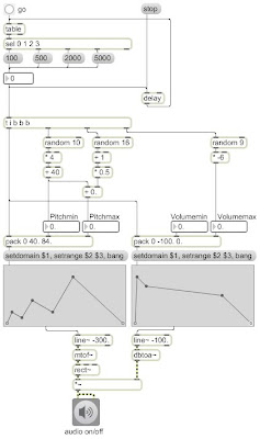
The shapes stay the same, but their transformations are chosen pseudo-randomly within specific ranges. The durations, which are also used as the delay time before starting the next shape, are chosen from among four possibilities: 100 ms, 500 ms, 2 sec, or 5 sec. The first duration will cause very short notes in which the envelope functions just have a timbral effect. The second duration is also a short note length (1/2 sec), but is just enough time for us to make out the shape within the note. The next two durations are definitely long enough for us to track the shape of the control functions as they affect pitch glissando and volume over the duration of a short "phrase".

The durations are chosen using a distribution of probabilities. An important thing to notice about probabilistic choices of durations is that long durations take up much more time than short durations. So if we used an equal distribution of probabilities, the long notes would take up way more of the total time than the short notes, and it would give the effect of the long notes predominating. The proportion of the given durations is 1:5:20:50, so if each duration were chosen with equal likelihood, the 2-second and 5-second notes would take up 70/76 (92.1%) of the total time. To counter that effect, we can use a distribution that is the inverse of the proportions of the note durations. (See inside the table object.)

As in the earlier cited example, we use function objects to draw the function shapes, for each note we set the range and domain to the desired values, and then we bang the functions to cause them to send their information to the line~ objects.

It's important to note that in this example, instead of the line segment functions controlling frequency and amplitude of the synthesized sound directly, they control the subjective parameters pitch and volume, specified as MIDI note names and decibels, respectively. Much has been written on the logarithmic nature of subjective perception relative to empirical measurement. This is particularly demonstrable in the case of musical pitch and loudness. We perceive these subjective traits as the logarithm of the empirical sonic attributes called fundamental frequency and amplitude. Fortunately, that logarithmic relationship makes it fairly easy to do a mathematical translation from a linear pitch difference or loudness difference into the appropriate exponential curve in the physical attribute of frequency or amplitude. The formula for translating MIDI pitch m into frequency f, according to the 12-notes-per-octave equal-tempered tuning system is f=440(2^((69-m)/12)). Using the reference frequency of A=440 Hz, which is equivalent to MIDI note number 69, multiply that times the (69-m)/12th root of 2. Max provides objects called mtof (for individual Max messages) and mtof~ (for signals) that do this math for you. The formula for translating volume in decibels d into amplitude a is a=10^(d/20). The amplitude a is calculated as 10 to the power of (d/20). This makes a reference of 0 dB equal to an amplitude of 1 (the greatest possible amplitude playable by Max signal processing), and all negative decibel values will result in an amplitude between 1 and 0. Max provides objects called dbtoa and dbtoa~ to do this math for you.

The arguments in the line~ objects might look a little strange, and they're not very important; they were chosen just to keep the program from making any sound when it's first opened. There's not really a MIDI pitch number that corresponds to a frequency of 0 (which would stop the rect~ oscillator)--MIDI pitch number 0 is a super-low C that would actually have a fundamental frequency of 8.1758 Hz--but -300 is a hypothetical MIDI number that would slow the oscillator down to about 0 Hz. Similarly, there is no decibel value that would truly give an amplitude of 0 (it would have to be negative infinity!), but -100 dB is equal to an amplitude of 0.00001, which is for all practical purposes inaudible.

Now let's look at the actual numbers being used for the pitches and volumes. The volume (peak amplitude) of each note will be one of nine possible decibel values, ranging from 0 dB (fff) to -48 dB (ppp) in increments of 6 dB. That's a pretty wide dynamic range for the peak amplitudes; it's at least as wide as most instrumentalists habitually use. Of course, recording systems need a much wider range than this to record all the subtleties of sounds in their quietest moments, but I'm just referring to the dynamic range of the peak amplitudes (the attacks) of the notes. The low end of the pitch range for each note will be one of 10 possible pitches, ranging from E just below the bass staff (MIDI 40) to E at the top of the treble staff (MIDI 76), in increments of a major third (4 semitones). The size of the range (the difference between Pitchmin and Pitchmax) will range from 0.5 to 8 semitones (from 1/4 tone to a minor 6th), as measured in 16 quarter-tone steps. This gives a possibility of some relatively wide glissandi and some very subtle small ones.

To test this program, just start the audio and click on the go button. Notice that most of the notes are very short (100 ms or 500 ms), with occasional longer notes (2 sec or 5 sec). The dynamics are arbitrarily and equally distributed from ppp to fff, and the pitches are arbitrarily and equally distributed from low to high, with a variety of glissando ranges.

My contention is that even though the compositional decisions made by the computer are arbitrary and undistinguished in their own right, there is a sense of unity and consistency to the sounds being played, due to the constant use of single shapes for pitch glissando and amplitude envelope, and that this helps to give an impression of coherency and intentionality. That is presumably the main utility of motive in composition: it gives a sense of repetition, recognizable variation, and consistency to a variety of different sounds.

Line-segment control function

In the article on fading by linear interpolation, you can see a demonstration of how a particular characteristic of a sound or an image (such as the amplitude of a sound or the brightness of an image) can be modified gradually over time. A word that's important for this type of operation is parameter, which means a numerical descriptor of a characteristic. For example, amplitude and brightness can each be controlled by a single number representing "gain" (the factor by which we turn it up or down). In that example using a "gain" factor to control amplitude or brightness simply involves multiplying the signal (the thing you want to modify) by the gain factor. In the case of audio, we multiply every single individual sample of the audio signal (tens of thousands of samples per second) by the gain factor; in the case of video we multiply every color value of every pixel of every frame by the gain factor. (That is exactly what the "brightness" operation is doing internally in the jit.brcosa object.) In each case, a single number sets a precise amount by which we modify a particular parameter. When discussing a sound or an image or a musical passage or a video, there are often many characteristics that can be usefully described by a number. When you get right down to it, it's usually possible to convert nearly any description into one or more numbers somehow, and once you've done that, the description can then be manipulated by arithmetic operations.

So, as we saw in that example, when a parameter changes over time, it can create an interesting change in aesthetic effect (such as a fade in or out). The change in that case was linear and directional. That makes for a simple yet clear and direct type of change. You can think of the straight line as one simple kind of shape imposed on the characteristic being controlled. Other shapes such as smooth curves or irregular patterns are also possible.

Before we go on, let's define a couple of words: the nouns control and function.

A control is something that we don't perceive directly, but the effect of which we can perceive when it's applied to a parameter. For instance, in the fading by means of linear interpolation example, we don't literally see a line or hear a line, but we perceive the linear effect when the line is applied to the gain factor that controls brightness and amplitude.

A function is a defined relationship between two variables. Let's call those variables x and y, which could stand for anything. In general one variable, x, stands for something "given" or "known" (an example might be time, which we can know with some accuracy using a clock), and the other variable, y, stands for something the value of which will depend upon the value of x. We say that "y varies as a function of x", which means that there is a known relationship that permits us to know the value of y if we know the value of x. Often the relationship between x and y can be perfectly described by a mathematical equation that contains two variables, x and y. That's what mathematicians generally mean when they use the word function: an equation that permits you to calculate the value of y for every possible value of x you might put into the equation. That's what's being described by the examples in the article on the mathematical manipulation of digital media. The formulae such as y=x, or y = Asin(2πƒt+ø)+d, or y=mx+b are examples of functions in which the value of y depends on the value of x in a way that can be reliably calculated. If we plug many different values of x into the equation and calculate y for each one, and graph the results with x on the horizontal axis and y on the vertical axis, we'll get a shape. That shape is called the "graph of the function". But a mathematical equation is not the only way to define a relationship between two variables.

A function could also be a shape that is not easily described by a mathematical equation, and we would discover the value of y by mapping it to its corresponding x value on the graph. Another way would be to actually have a listed series of all possible x values and the y values that correspond with them. These methods may take a bit more memory to store a complex shape or a list of x,y pairs, but a) they allow us to use shapes that are not easily described mathematically and b) rather than requiring calculation, they just require a quick lookup of the y value based on the known x value.

But regardless of the precise method of establishing the relationship between the known variable and the unknown variable--whether it's done by a calculation or a lookup--one important characteristic of a function is that it describes a knowable one-to-one relationship (of any degree of complexity) between x values and y values.

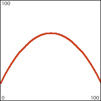
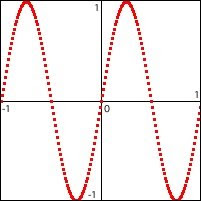
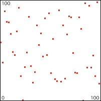
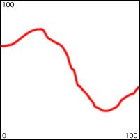
So, by combining those two words, we arrive at an expression that is used frequently in audio sound synthesis, and which, as we will see, can also be used in algorithmic composition: control function. A control function is a shape that is used to control a parameter in sound or music or video or animation. Most commonly x is the passage of time, and y is the value of some parameter over that period of time. All kinds of shapes are potentially useful as control functions.

Straight lines

Curves

Trigonometric functions

Random or arbitrary x,y pairs

Freehand drawn shapes

Combinations of line segments

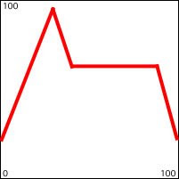
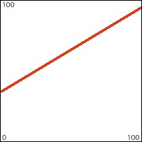
We'll look at how some of these control functions can be used to control or modify sounds, and then we'll transfer some of that thinking into the control of attributes of a musical structure or an animation. We'll start with line segment shapes such as the one depicted directly above.

The article on linear change introduces some of the math involved in making a formulaic description of linear change over time, and the article on linear interpolation introduces the handy Max object called line. The line object lets you just specify a destination value (the value you want to get to), a transition time (how long you want to take to get there), and a reporting interval (how often you want it to send out intermediate values along the way there), and it sends out a timed series of values that progress linearly from its current value to the destination value in the specified amount of time. Max also provides a line~ object for doing the same thing for an audio signal. The messages you send to a line~ object differ from those of line in two significant ways. First of all, there is no argument for the "reporting interval" in line~ because line~ sends out an audio signal, and every single sample of that signal reports an intermediate value interpolated between the starting value and the destination value; in effect, the reporting rate is the same as the audio sampling rate. So all line~ really requires is two numbers: the destination value and the transition time. The other difference is that line~ can receive multiple value-time pairs in the same message, all as part of the same list. For example, a message such as '1. 1500 0.5 500 0.5 2000 0. 6000' will cause line~ to send out a signal that goes to 1 in 1500 milliseconds, goes from 1 to 0.5 in 500 milliseconds, stays at 0.5 for 2000 milliseconds, goes to 0 in 6000 milliseconds, and stays at 0 until it receives a message causing it to go to a different value. In this way a single message can describe a function over time made up of several straight line segments.

The function object allows the user to draw a line-segment shape of this sort. When the object receives a 'bang' it sends out such a message (intended for line~) that will cause line~ to send out that function shape. The minimum and maximum of the range (of the y axis) of the function can be set by a 'setrange' message, and the duration (of the x axis) can be set by a 'setdomain' message.

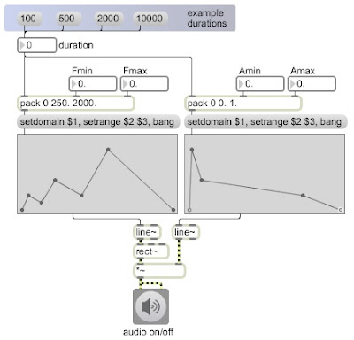
This patch shows the use of line segment control functions to shape the frequency and amplitude of a tone. When you choose a duration for the function, that number is used to set the domain of the function objects (and also uses whatever values have been chosen for the minimum and maximum of the frequency and amplitude ranges).

For the amplitude function, a shape has been chosen that is similar to the amplitude envelope of many instruments when the function takes place over a duration of about 500 to 2000 milliseconds. For the frequency function, a shape has been chosen that results in three up-down glissandi that increase in range and duration. Try listening to these control functions at different durations. When played very slowly over 10 seconds, the envelopes are clearly audible as gradual frequency glissandi and amplitude changes. When played over a quicker duration such as 1/2 second, the amplitude envelope sounds quite natural and the glissandi are quick and almost melodic. When played extremely fast, over 1/10 of a second, the glissandi are too fast to perceive as such, and the effect is mostly timbral. Try also changing the frequency range values to see what effect occurs when the range is very small or very large.

The point here is that the same functions can be "stretched" (augmented or diminished) over a variety of durations and/or ranges to create a wide variety of sonic/musical effects without changing the basic shape of the control functions. One can thus think of a distinctive control function shape as being analogous to a musical motive or formal structure. The same motivic shape can occur over a long period of time (phrase level), or a short period (note level), or an extremely short period (for timbral effect). In this program, one can also simply draw a new control function with the mouse, to create a new motive.