
So far we've used numbers to describe and compare amounts of time and rates of speed, to count and enumerate, to index orders of events, and to indicate musical pitch, loudness, intensity of color, and position in a two-dimensional coordinate system. Composition and aesthetic appreciation are about the creation and recognition of patterns--sonic, temporal, visual, and rhetorical. Thus, to the extent that we can program a computer to generate interesting numerical patterns, we are on the path to computer-generated art.
Mathematical functions with two variables (such as x and y) can be graphed in two dimensions as a curve. If we consider one of the variables, x, to be the linear progression of time, then the shape of the curve displays the change in the other variable, y, over time. Almost any function with two variables is potentially useful for algorithmic composition of time-based media art (music, video, animation, etc.), if we just consider one variable to be the passage of time and the other variable to describe some characteristic of the art.
Let's look at some examples. Remember x will stand for the passage of time, and y will stand for the value of something else. Time is expressed in some arbitrary units; you can think of the units as seconds for now. Likewise y is some arbitrary thing we're measuring; for the sake of having both a sonic and a visual example, let's think of y as standing for the volume (loudness) of a tone or the brightness of a color.
What does this formula tell us?
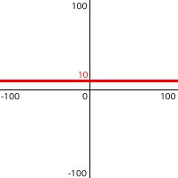
y = 10
Well, there's no x in that formula. That means that y is independent of x. No matter what x is, the value of y will always be 10. This describes a constant value, not a variable one. y stays constant over time. If this were loudness or brightness, we would perceive no change.
Now how about this formula?
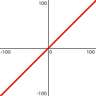
y = x
This means that y increases as time progresses. Since time progresses linearly, y will increase linearly. If we call the start of the time under consideration "time 0", meaning x = 0, then y will be 0 at that time. At time 10, y will be 10, and so on. So over the course of time going from 0 to 10, y will increase linearly from 0 to 10. The units we're using are arbitrary, but imagine that over the course of 10 seconds the volume of a sound fades in from 0 to 10, and a color fades from total darkness to a brightness of 10. As soon as we get to real examples, we'll have to concern ourselves with what the units actually are and what they mean, but for now we're just talking abstractly.
Here's a formula that gives a simple curve.
y = sin(2πx)
This causes y to vary up and down in a smooth, sinusoidal fashion. Of course, all of these formulae are rather oversimplified; we'd need to provide more numerical information to make x and y have the right values for the particular usage to which we're applying them. But these simple examples show that we can generate curves by tracking any two variables, and that by increasing x linearly to stand for the passage of time we can use the resulting y to control some aspect of digital media
.jpg)
We can add other constant numbers or variables into the formula to make adjustments that bring the y value into a desired range. Those additional constants or variables will usually do one of two things: either scale the x or y value by multiplication (multiply it by some amount to scale it to a larger or smaller range) or offset the x or y value by addition (add some amount to it to push it into a different region).
For example, a more complete and useful formula for generating a smooth sinusoidal change would look like this.
y = Asin(2πƒt+ø)+d
where A is the amplitude of the sinusoid, ƒ is its frequency, t is time, ø is its phase offset, and d is its DC offset. The variable t in this case is like x in the previous examples. ƒ scales the sinusoid on the horizontal axis, and A scales it on the vertical axis; ø allows us to offset the sinusoid on the horizontal axis, and d will offset it on the vertical axis. We'll use some version of this formula often in synthesizing and processing sound in future lessons.
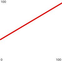
Here's a simpler equation, that permits us to make any desired linear variation in y.
y = mx+b
where m is the slope (steepness of the angle) of the change in y, and b is the y intercept (the y value at which the line intersects the y axis), which we can call the (vertical) offset. Here's what that would look like with m = 0.6 and b = 36.

Since we will be starting things at time 0, and will be mostly dealing with non-negative y values for MIDI, color, coordinates, etc., it sometimes makes sense just to think about the upper-right quadrant of the graph, showing y values as x (time) increases from 0.
In the next lesson we'll put the y=mx+b equation into practice in a program.
2 comments:
Hi Chris. I'm studying your posts and I think I caught a type-o.
"y = mx+b
where x is the slope (steepness of the angle)"
-T
Right you are. Thanks. Fixed it. -C
Post a Comment