Sunday, August 31, 2008

Randomness

What does it mean to say that something is random? In general everyday usage it means a thing that occurs or is chosen without any particular bias, method, or conscious decision. In statistical usage it means equal likelihood of all possibilities. Both of those usages are applicable in the case of a card trick that begins, "Pick a card, any card." If the cards are presented in a neutral way, and the chooser is at liberty to choose any card, then all cards are equally likely to be chosen. And in most cases the chooser chooses at random, too, with no particular method or preference.

In all real world instances of randomness, we're not really talking about all possibilities; there is a limited range or field of possibilities. In a deck of cards, for instance, there are 52 possibilities (not counting jokers), each with a unique designation such as "three of hearts". So for each card there is a 1-in-52 chance of being the chosen card, and we know that it will have one of an expected set of designations. (There is no chance of, let's say, choosing a 57th card with the designation "seventeen of swords".) It is a limited number and type of possibility, but within those established limits randomness can occur.

True randomness is thus more of a concept than a reality. In computer programming, when we refer to random numbers, we actually mean pseudo-random numbers: numbers chosen from within a particular range of equally likely possibilities, by some system that is too complicated or obscure for us to comprehend, resulting in choices that appear to have no governing bias, method, or pattern. All programming languages contain a function for generating pseudo-random numbers--numbers within a particular range that appear to be completely unpredictable and to have no over-all pattern. (Mathematicians and computer scientists have devised many methods for generating pseudo-random numbers, but we won't concern ourselves here with the method of generation. We'll simply use the method provided for us by the programming language we happen to be using.)

Choosing a random number in a computer program (i.e., generating a number within a known set of possibilities by a pseudo-random process) is a way to simulate arbitrary decision making (a decision made without method or preference). It's also possible to program the computer to make arbitrary decisions using so-called weighted (i.e., unequal) probabilities, such that some numbers occur statistically more often than others (given a large enough statistical sample). We'll look at weighted randomness in another lesson. For now, we'll stick to random numbers of equal probability.

This program demonstrates some methods of random number generation in Max. It uses those random numbers to select sounds and images arbitrarily from limited sets of possibilities. For this program to work properly, you'll also need to download the very small audio clips and images that it uses. Just right-click (or control-click on Macintosh) on the following links, and save the files in the same directory as you save the program itself.
Images: gourmet.jpg, nubleu.jpg, brascroises.jpg, guitariste.jpg, tragedie.jpg, celestina.jpg
Sounds: bd.aif, tom.aif, snare.aif, hihat.aif, cymbal.aif


To begin discussing randomness in programming, let's stay with the "pick a card, any card" example for a moment. The key to the statistical definition of randomness, you'll recall, is that there is an equal likelihood of each possible outcome. In other words, there is an equal probability of each possible result. That leads us to the mathematical definition of probability: the number of looked-for results divided by the number of possible results. If we choose at random from 52 possibilities, there is a 1-in-52 chance of any particular looked-for result (such as the ace of spades, for example); that means the probability of choosing the ace of spades (1 looked-for result) out of all possible cards (52 of them) is 1/52, which is 0.019231. The probability of choosing any other particular card is the same. Note that by this definition of probability, the probability of any particular outcome (or set of looked-for results) can be expressed as a fraction from 0 to 1 inclusive, and the sum of the probabilities of all the possible results will equal 1.

If we put the chosen card back in the deck, and mix the cards up again, we'll once again have 52 cards, all of equal probability 0.019231. If on the other hand, we set the first chosen card aside instead of putting it back in the deck, and now choose from the remaining 51 cards, the first chosen card will now have a 0 probability of being chosen (it's no longer a possibility), and all the remaining cards will have a probability of 1/51, which is 0.019608. You can see that as we remove more cards from the deck, the probability of choosing any particular one of the remaining cards will increase, although all remaining cards will still have an equal probability. By the time we make our 51st choice, we'll be down to only two remaining cards, each with a probability of 0.5, and on the 52nd choice we'll have a 100% likelihood (a probability of 1) of choosing the one remaining card.

The distinction in the preceding paragraph between putting the chosen card back in the deck or not is an illustration of the difference between the random object and the urn object in Max. The random object chooses from a specified number of possible integers, with each choice being independent of any and all previous choices. The urn object also chooses at random, but it never repeats a choice; once it has chosen a certain number, that number is taken out of the set of possible choices (until the object is reset to its initial state with a clear message). Thus, urn avoids repetitions, and once it has chosen each possibility once, it stops choosing numbers, and instead sends a bang out its right outlet to report that all possible choices have been made. The random object, by contrast, always "forgets" its previous choice, and chooses anew from all of the numbers within the specified range.

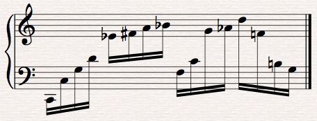
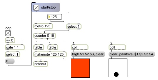
In this example program, program No. 1 chooses randomly from a list of twelve stored chords every two seconds. The chords are composed in such a way that they have a clear root and all can be reasonably interpreted to have a function in C minor, yet they are sufficiently ambiguous and are voiced in such a way that any chord can reasonably succeed any other chord.

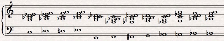
Because the ordering of the chords is chosen at random--truly arbitrarily--by the program, the harmonic progression sounds rather aimless. That's because it is, in fact. The program has no sense of harmonic function, no rules about one chord leading to or following another, etc., the way that a human improviser would. So this type of arbitrary decision making at this formal level can't really be likened to compositional or improvisational decision making that a thinking human would perform. It's useful for producing unpredictable ordering of a set of events, though, and its effectiveness varies at different formal levels and with different types of controls and applications, so we'll see different uses of random numbers in future lessons.

The random object needs to be supplied with a number that specifies how many possible numbers it can choose from. Since this random object has the argument 12, it will choose from among 12 different numbers, integers 0 to 11. The random object always chooses numbers from 0 up to one less than the specified limit. This results in the right number of possibilities, and the fact that the range starts at 0 makes it useful for accessing arrays, as we've seen in earlier examples. It also means that we can easily change the range by adding some number to the output of random. Because each random choice is independent of previous choices there is a possibility--indeed there is a 0.083333 probability--that it will choose the same chord twice in a row.

The chords are stored as twelve 5-note lists in coll, indexed with numbers from 0 to 11. When these lists come out of coll they get broken up into five individual messages by iter so that they can be sent out as five separate--but essentially simultaneous--MIDI notes.

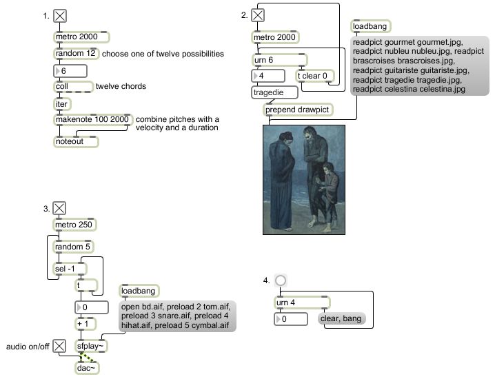
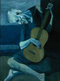
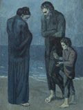
Program No. 2 uses urn to choose a random ordering of six images. Like the twelve chords, the images have been selected because they are related--they're all images of human subjects from Picasso's blue period--but there is no aesthetic or logical reasoning behind the order in which they're presented. The urn object ensures that there are no repetitions, and after it has chosen each of the six the possible numbers from 0 to 5, the next time it gets a bang from the metro it sends a bang out its right outlet to indicate that all possibilities have been expended. In this program, we use that notification to turn off the metro and to send a clear message back to urn to get it ready for the next time.

The program initially reads into memory each of the images we want to display, and assigns each of them a symbolic name. Those names are also stored in a umenu object so that they can be recalled with the numbers 0 through 5. When urn sends out a number, umenu uses the number to look up the name stored at that index in its internal array, and sends the name out its middle outlet. The prepend object puts the word drawpict before the name, so that a message such as drawpict guitariste will go to the lcd object and draw the picture.

Program No. 3 shows a slight variation on the sort of random selection used in No. 1. It plays very short sound files chosen at random from five possibilities, but never plays the same file twice in a row. Each time that a random number comes out, it goes to a select object to be compared to the previous number. If it is not the same as the previous number, it is passed out the right outlet of select and used to choose a sound. However, if it is the same as the previous number, select sends a bang back to random to try again. The select object is initialized with the argument -1 so that the first choice by random, which we know cannot be -1, will never be rejected. So after the very first choice, instead of there being five possibilities, there are actually only four, because we know that the preceding number will be rejected if it's chosen again immediately. It's still random, but with a rule imposed after the choice, a rule that rejects repetitions and keeps retrying until it gets a new number.

[N.B. This programming technique of using an object's output to potentially trigger immediate new input back to its left inlet is not generally advisable in Max, because it could cause a "stack overflow", a situation in which Max is required to perform too many tasks in too short a space of time. However, in this case, the probability that random would choose the same number enough times in a row to cause a stack overflow is minuscule.]

The program initially opens each of the different sound files we will want to play and stores a pointer to each of those files as a numbered "cue". Because of the way that the sfplay~ object is designed, the sound file most recently opened with an open message is considered cue number 1, and other numbered cues can be specified with the preload message. There is no cue number 0 in sfplay~; that number is reserved for stopping whatever cue is currently playing. Therefore, what we really need in order to access the five cues in sfplay~ is not numbers 0 through 4, but rather numbers 1 through 5. This is easy to achieve simply by adding 1 to every random number before passing it on to sfplay~ to be used as a cue number. (This addition is another example of an offset, as demonstrated in the earlier examples on linear mapping.)

Program No. 4 just demonstrates a handy trick for causing urn to keep outputting numbers once it has chosen all the possibilities. You can use the notification bang that comes out of urn's right outlet to trigger some new action, so in this example we use it to trigger a clear message back to urn itself, then retry with a new bang to urn. Note that this leaves open the possibility of a repetition between successive numbers, since the first new number that urn chooses after it is cleared could possibly be the same as the last number it chose before it was cleared. (The probability of an immediate repetition occurring in this way is inversely proportional to the number of possibilities.)

Notice that the complete randomness produced by random leaves open the possibility of some improbable successions of events occurring. Unlikely short-term patterns, such as 2,2,2 or 1,2,1,2 are possible, especially when the total number of possibilities is relatively small. So random is useful for generating unpredictable results, but that includes the possibility of improbable distinctive successions. The urn object avoids such successions that involve repetition of a number, but it becomes more predictable as its number of possible choices decreases. (We know that it won't choose a number that it has already chosen.)

The artist-programmer should determine what sort of randomness, if any, meets the aesthetic goals of a particular situation. Future lessons will show other uses of random numbers for decision making.

Friday, August 29, 2008

Fading by means of interpolation

To reinforce the importance of linear interpolation, let's look at a common technique used in music and video, the fade.

Fading a sound in from silence, or fading it out to silence, or fading an image in from darkness, or fading it out to darkness--these are commonly-occurring gradual transitions of the sort discussed in the previous lesson on linear change. To give the sense of gradual change between one value and another, which we abstractly called point A and point B in the previous lesson, we need for the program to calculate intermediate values to create a linear transition. In the previous example, the transition was a simultaneous linear change in pitch (MIDI key number, from low to high) and loudness (MIDI velocity, from high to low) of musical notes. Now we'll do the same thing with loudness of a sound and brightness of an image.

This program shows an automated fade-in of sound and image by means of linear interpolation.

For this program to work properly, it needs to be able to access a particular (very small) image file. You should download the file tinyocean.jpg and place it in the same folder as the program file.

Whereas the previous examples on linear interpolation used the objects clocker and expr to calculate linear progressions of values, in this example we take advantage of the Max object line, which does essentially the same thing but takes care of some of the math and programming tasks for you. The line object outputs a linear progression of values that arrive at a specified destination value in a specified amount of time. It receives in its inlet a destination value (the value at which it should eventually arrive), a transition time (how long it should take to get to the destination value), and a time interval (how often it should send out an intermediate value as it progresses toward the destination. It takes care of the scheduling of output and stops when it reaches its destination. [N.B. The line object has a slightly quirky way of calculating timing, which you should be aware of. You can read about it in the "line_timing_tricks" subpatch of the line object's help file.]

Some of the earlier lessons have used MSP audio, but this is the first one that uses Jitter visual display. (MSP object names all end with the ~ character and Jitter object names all begin with the jit. prefix. MSP objects calculate a constant stream of audio samples, and Jitter objects store and process and display multi-dimensional arrays of data (one of the most common of which is a two-dimensional array of color data to display a still image or a frame of video). For MSP audio to work, MSP must be turned on explicitly somewhere in the program; and for time-varying images to be displayed in Jitter, the data must be continually sent to a display wihdow, usually triggered by a metro set to a fast tempo (less than or equal to the desired frame rate). This is explained in the very first chapter of the MSP and Jitter tutorials that come with the Max program. That's what the toggle switch in the upper-right corner of the program does; it starts MSP audio via the dac~ object and starts a metro that triggers repeated recalculation and display of the image. The metro and dac~ objects both need to be turned on for the program to work.

When the audio and video are turned on, we don't hear or see anything because the amplitude of the sound is turned to 0 (the default value of the line~ object is 0) and the brightness of the image is set to 0 (with the @brightness 0 attribute typed into the jit.brcosa object. The image is automatically loaded into a Jitter matrix (the jit.matrix object) when the program is loaded. So everything is initialized correctly automatically when the program is opened. Once the audio and video has been turned on, MSP is calculating audio, but all the samples end up being 0 (because the *~ object is multiplying every sample by 0); and Jitter is calculating the video display at a rate of 25 fps, but all the pixels end up being black (because the jit.brcosa object is multiplying every pixel by 0). To fade the sound and image in, then, we just need to create a gradual progression of values that increase upward from those initial 0 values.

When you click on the button, it triggers two messages to the line object that will change the brightness of the image. The first message, set 0., resets line internally to that value. The second message, which comes immediately after, 1. 5001 40, says "Go toward 1, arriving there in 5001 milliseconds, sending out an interpolated value between 0 and 1 every 40 milliseconds." Since 40 ms is the same periodicity as the metro, every "frame" of the video display will have a slightly greater calculated brightness over the course of 5 seconds, till it reaches a full brightness of 1. (Every pixel in the image gets multiplied by the brightness factor each time.) At practically the same time, two messages are sent to the line object that will change the loudness of the sound. The first message resets line internally to a value of -78, and the immediately ensuing message tells line to go toward -18 over the course of 5 seconds, sending out an interpolated value every 40 ms. These values are treated as decibels of amplitude, and are converted into actual linear amplitude values by the dbtoa object. The line~ object is similar to line, in that it requires a destination value and a transition time; however, it does not require a time interval for reporting, because it interpolates constantly for every single audio sample (i.e., at the audio sampling rate).

The three message boxes in the yellow panel are for "clean-up": for resetting things when the audio and video are turned off by the toggle at the top of the program. The select 0 object detects when the toggle has been turned off, and triggers a stop message to both of the line objects, just in case they are in progress, a 0 message to reset the amplitude and brightness values to 0, and a bang to trigger the image once more (with the brightness of 0, thus displaying a black screen). This clean-up makes sure everything truly is (and looks, and sounds) turned off.

Both in the case of brightness and the case of loudness (amplitude), multiplying by some number scales the value; multiplying by 0 reduces everything to 0, multiplying by some number greater than 0 but less than 1 reduces it to less than its normal amount, multiplying it by 1 leaves it alone, and multiplying it by a number greater than 1 will increase it.

There is an aspect of our perception of audio that complicates matters a bit, which is that we actually perceive loudness and pitch subjectively as the logarithm of relative amplitude and frequency. That is to say, our perception of sound intensity and musical pitch requires that the amplitude and frequency change in a geometric progression (i.e. multiplicatively) in order for us to perceive the change as an arithmetic progression (i.e. additively). We'll discuss this more in future chapters. For now, it's enough just to note that when we are concerned with the perceived loudness of a sound, it's often best to discuss its amplitude in terms of decibels (a logarithmic formula for characterizing relative amplitude). That's what the dbtoa object does for us; it allows us to make a linear progression stated in decibels and calculates an appropriate exponential increase in amplitude.

Just to illustrate, -78 decibels is equal to an amplitude of 0.000126, and -18 decibels is equal to an amplitude of 0.126. So in our fade-in of the noise in this example, the amplitude increases by a factor of 1000 (but by an additive difference of 0.125874). If we make a linear progression in decibels from -78 to -18, when we're halfway there we'll be at -48 dB, which is an amplitude of 0.004. Although that's much less than halfway to 0.126 arithmetically, 0.004 has the same ratio relationship to 0.000126 as 0.126 has to 0.004, so we're halfway there in terms of perceived loudness. If, on the other hand, we made a straight linear progression in amplitude from 0.000126 to 0.126, at the halfway point we would be at 0.0628, which is half the amplitude we are heading for, but is 500 times the amplitude at which we started! In other words, over the first half of the period of time, the amplitude would increase by a factor of 500, but for the second half of the period of time it would increase by a factor of only 2. We would hear a very substantial change in the first half, and very little change in the second half. The decibel scale corresponds much more closely to our subjective perception of a sound's intensity, and thus gives us a fade-in that feels more linear to us.

And finally, an aesthetic observation about the relationship of sound and image. The white noise (total randomness of audio samples) produced by the noise~ object is related to the noise made by the turbulence of ocean waves. Its not exactly the same, of course, but when the sound and the image are juxtaposed, and are further linked by the way they fade simultaneously, the visual image may influence us to feel that the noise is somehow ocean-like (even though it was not produced by an ocean) and the sound may serve to enhance the evocative appeal of the image. When two things are juxtaposed, our tendency is to think about their relationship, which sometimes includes finding relationships that may not in fact be there.

Tuesday, August 26, 2008

Linear change

"The shortest distance between two points is a straight line." That mathematical truism recalled from our geometry class is often quoted as a sort of proverb, reminding us that the most direct way to get somewhere is usually to head straight for it. The straight line stands for directness, and we can easily perceive its direction and predict where it will arrive if it continues. Thus, straight lines are useful for describing gradual-yet-direct change. If we draw a straight line from point A to point B, we're getting there by the most direct route, and we're also drawing every intermediate point that lies directly between A and B.

In the previous lesson, we provided the formula y=mx+b as a general way to describe any line. That's how it's given in arithmetic textbooks, but we'll need to rephrase it a bit for our purposes. For starters, how do we calculate the slope m? Well, for any two points--we'll call them A and B--we can calculate the slope of the line that runs through them (and thus the line segment that connects them) by dividing the vertical distance between them by the horizontal distance between them; that is to say by dividing the difference in their y values by the difference in their x values. So if the coordinates of point A are (xa, ya) and the coordinates of point B are (xb, yb), then the slope m is equal to (yb-ya)/(xb-xa). To refer to the last example from the previous lesson, the first point on the line segment is (0,36) and the last point is (100,96). so the slope of the line is (96-36)/(100-0), which is 60/100, which is 0.6. Thus, by knowing the slope m (0.6) and the offset b (36), we can calculate what y value will lie on the line for any x value we put into the formula.


In practical terms, for the purpose of programming linear change in sound, music, video, animation, etc., we'll need to know those values, or at least we'll need to be able to calculate them. (In the above example, we were able to calculate the slope because we knew the starting and ending x and y values.) Then, by starting at the desired value for x (a starting point in time) and proceeding to a desired destination value for x (a future point in time), we can calculate the values for y for as many intermediate x points as we want, to give the impression of a linear change in y. Before we look at an example, let's consider two other terms that are commonly used in digital media arts, which have direct relevance to this definition of a line.

-----

The term linear interpolation between two points A and B means finding an appropriate intermediate point (or points) that would exist if there were a straight line between A and B. To continue with the example we've been using, if we have the two points (0,36) and (100, 96), we can interpolate one or more points between them by calculating the y value at a hypothetical x value between 0 and 100. For example, just by using the formula and the known values for slope and offset, we can calculate that when x equals 20 y will equal 48, and when x equals 80 y will equal 84.
(0.6)20+36=48
(0.6)80+36=84
So, for any point between A and B, we can interpolate one or more additional points that will lie on a straight line segment between them. Another way to say this is that for any intermediate x value, we can find the appropriate corresponding y value.

Tangent: There's another way to think of linear interpolation, which is to think of "how far along" the intermediate x is, on a path from point A to point B. In other words, for the hypothetical x value, how far is it from its starting point xa, and how far is it from its destination point xb? We can actually calculate it as a fraction between 0 and 1 by calculating its distance from xa, which will be x-xa, and dividing that by the total distance between xa and xb, which will be xb-xa; so the fraction of the distance that a hypothetical x is on the path from xa to xb can be calculated with the expression (x-xa)/(xb-xa). So another way to think about calculating the y value for a hypothetical x value, is to multiply the destination y (yb) by that fraction because we're that fraction of the way there, and multiply the starting y (ya) by 1 minus that fraction. The equation for finding the y value that corresponds with a hypothetical x value is thus y=(yb(x-xa)/(xb-xa))+(ya(1-((x-xa)/(xb-xa))). Or, to put it a bit more simply, y = ((x-xa)(yb-ya))/(xb-xa)+yb. That's a valid formula for linear interpolation, or linear mapping of x to y.

This process of linear interpolation is thus very closely related to another term, linear mapping, which means making a direct correlation of an x value to its corresponding y value. If we have a given range of x values (say, from xa to xb), and a corresponding range of y values (say, from ya to yb), then for any value of x we can calculate the linearly corresponding y value. This is called mapping x values to y values. (In theory, there could be a wide variety of curved or non-linear "maps" by which we make these correlations between x values and y values, however, for now we'll stick to linear mapping.) The formula for linear mapping, if you needed to program it yourself, is shown in the preceding paragraph. Mercifully, Max provides many objects that can calculate mapping for you, such as zmap, scale, etc.), but it's important to understand mapping conceptually since it is key to all sorts of programming in digital media.

-----

Now let's look at a simple example of linear change. This program plays musical notes every 80 milliseconds (i.e., at the rate of 12.5 notes per second) for 2 seconds (2000 milliseconds). Over the course of those two seconds, the pitch of the notes changes linearly from MIDI 36 (low C) to MIDI 96 (high C) and the MIDI velocity (loudness) of the notes changes linearly from 124 (fortissimo) to 32 (piano). The result is a program that plays an ascending pentatonic scale, with a diminuendo.

Note that the program plays a major pentatonic scale, which is not a strictly linear configuration. (Some steps are 2 semitones, and some are 3 semitones.) Because we're stepping through five octaves of pitch in 25 increments, each step should be 1/5 of an octave. However, because MIDI does not allow for fractional values, the decimal part of the intermediary pitch values is truncated (chopped off), so ultimately not all the steps are exactly the same size. The fortuitous result of this truncation is the pattern that gives a major pentatonic scale. There's no magical mathematical relationship between truncation and this particular pitch pattern. It's just a fortunate (calculated) coincidence of the range, the number of notes being played within it, MIDI representation of pitch, and truncation of the fractional part of the number.

Let's look at a couple of details in the program. The clocker object reports at regular intervals the amount of time elapsed since it was turned on. This is similar to the timed counting demonstrated with the metro and counter objects, but in this case it is counting in increments of a certain number of milliseconds, corresponding exactly to the amount of time that has passed. This is handy because it allows us to check each report to see if a certain amount of time has passed--in this case 2000 milliseconds--and do something at that time (in this case, stop the process). Since we know the desired stopping time (that is to say, the destination x value) we can also use each reported time to calcuate how far along we are to the destination time, and use that fraction for linear mapping of time to the pitch and velocity values.

We can divide the elapsed time (x) by the total time (2000) to get a fraction between 0 and 1. We then multiply that by the range of the desired y values (yb-ya), and add the desired offset (ya) to it. (We calculated the range of desired y values by subtracting the starting value from the ending value, i.e., yb-ya.) That's what's happening in the two expr objects. In the case of pitch, ya equals 36 and yb equals 96 so the range is 96-36, which is 60. In the case of velocity, ya equals 124 and yb equals 32 so the range is 32-124, which is -92. That's where the range values 60 and -92 come from in the expr objects. The numbers 36 and 124 in the expr objects are the ya (offset) values. The number boxes (because they are integer number boxes) drop the fractional part of the output from the exprs.

This direct use of the y=mx+b formula inside an expr object is just one way to do linear mapping in Max. The line object does automated linear interpolation, kind of like this combination of clocker and expr shown here, and other objects such as zmap and scale calculate mapping of x and y values if you provide the points A and B.

Linear motion, linear change, linear interpolation, and linear mapping are frequently used in composition and digital media.

Saturday, August 23, 2008

That's Why They Call Them Digital Media

The foregoing examples demonstrate that musical notes, colors, locations--and indeed anything else--can be described numerically. That's the essence of computational creativity, and the essence of digital intermedia/multimedia. Many of these lessons will be about exploring that way of systematically--and numerically--describing aesthetics and composition.

So far we've used numbers to describe and compare amounts of time and rates of speed, to count and enumerate, to index orders of events, and to indicate musical pitch, loudness, intensity of color, and position in a two-dimensional coordinate system. Composition and aesthetic appreciation are about the creation and recognition of patterns--sonic, temporal, visual, and rhetorical. Thus, to the extent that we can program a computer to generate interesting numerical patterns, we are on the path to computer-generated art.

Mathematical functions with two variables (such as x and y) can be graphed in two dimensions as a curve. If we consider one of the variables, x, to be the linear progression of time, then the shape of the curve displays the change in the other variable, y, over time. Almost any function with two variables is potentially useful for algorithmic composition of time-based media art (music, video, animation, etc.), if we just consider one variable to be the passage of time and the other variable to describe some characteristic of the art.

Let's look at some examples. Remember x will stand for the passage of time, and y will stand for the value of something else. Time is expressed in some arbitrary units; you can think of the units as seconds for now. Likewise y is some arbitrary thing we're measuring; for the sake of having both a sonic and a visual example, let's think of y as standing for the volume (loudness) of a tone or the brightness of a color.

What does this formula tell us?
y = 10
Well, there's no x in that formula. That means that y is independent of x. No matter what x is, the value of y will always be 10. This describes a constant value, not a variable one. y stays constant over time. If this were loudness or brightness, we would perceive no change.

Now how about this formula?
y = x
This means that y increases as time progresses. Since time progresses linearly, y will increase linearly. If we call the start of the time under consideration "time 0", meaning x = 0, then y will be 0 at that time. At time 10, y will be 10, and so on. So over the course of time going from 0 to 10, y will increase linearly from 0 to 10. The units we're using are arbitrary, but imagine that over the course of 10 seconds the volume of a sound fades in from 0 to 10, and a color fades from total darkness to a brightness of 10. As soon as we get to real examples, we'll have to concern ourselves with what the units actually are and what they mean, but for now we're just talking abstractly.

Here's a formula that gives a simple curve.
y = sin(2Ï€x)
This causes y to vary up and down in a smooth, sinusoidal fashion. Of course, all of these formulae are rather oversimplified; we'd need to provide more numerical information to make x and y have the right values for the particular usage to which we're applying them. But these simple examples show that we can generate curves by tracking any two variables, and that by increasing x linearly to stand for the passage of time we can use the resulting y to control some aspect of digital media


We can add other constant numbers or variables into the formula to make adjustments that bring the y value into a desired range. Those additional constants or variables will usually do one of two things: either scale the x or y value by multiplication (multiply it by some amount to scale it to a larger or smaller range) or offset the x or y value by addition (add some amount to it to push it into a different region).

For example, a more complete and useful formula for generating a smooth sinusoidal change would look like this.
y = Asin(2πƒt+ø)+d
where A is the amplitude of the sinusoid, ƒ is its frequency, t is time, ø is its phase offset, and d is its DC offset. The variable t in this case is like x in the previous examples. ƒ scales the sinusoid on the horizontal axis, and A scales it on the vertical axis; ø allows us to offset the sinusoid on the horizontal axis, and d will offset it on the vertical axis. We'll use some version of this formula often in synthesizing and processing sound in future lessons.

Here's a simpler equation, that permits us to make any desired linear variation in y.
y = mx+b
where m is the slope (steepness of the angle) of the change in y, and b is the y intercept (the y value at which the line intersects the y axis), which we can call the (vertical) offset. Here's what that would look like with m = 0.6 and b = 36.

Since we will be starting things at time 0, and will be mostly dealing with non-negative y values for MIDI, color, coordinates, etc., it sometimes makes sense just to think about the upper-right quadrant of the graph, showing y values as x (time) increases from 0.

In the next lesson we'll put the y=mx+b equation into practice in a program.

Friday, August 22, 2008

Analysis of Some Patterns

Let's examine some of the decisions that were made in composing the content for the example of counting through a list. The contents of the table and coll objects determine what pattern of notes, colors, or positions we perceive when we read through them.

The process of counting through a numbered array is independent of the contents of the array. The array could be an array of anything, and we could re-order or change the contents of the array and still employ the same process to read through it. So the counting process is necessary, but it's fairly uninteresting on its own. (At least, it's fairly uninteresting until we give it a more interesting rhythm than just reading at a constant rate.) The contents of the array are what's more important in determining the aesthetic of what is produced.

The program displays a sequence of 16 colors, 16 musical notes, and 16 positions for a black dot. Let's look at the colors first.

The color of the background of the lcd object is described by three numbers from 0 to 255 that state the value of Red, Green, and Blue in the mix. This is called RGB, and is one common way of describing colors digitally. The color values in the coll object were chosen to progress more-or-less directly through the color spectrum from red to green to blue and back toward red. Since there are 16 steps in the array, this naturally entails a few intermediate colors along the way. However, sixteen steps is way too few to give an impression of smooth gradual change; rather, we get a pattern of distinct colors that traverse the spectrum. And, if the program's looping feature is turned on, the pattern of colors seems to return fairly naturally to where it started.


The pattern of sixteen musical pitches is a little less direct, and a bit more complex. The first eight notes are an upward arpeggiation of the pitches C,C,G,D,Eb,F#,A,Bb, which could be thought of as a Cm13#11 chord. The next four notes are an upward arpeggiation of the pitches F,C,G,Ab, which could be thought of as an Fmadd9 chord (and/or, if we include the high D that comes next, as an Fm69 chord), and the final four notes are a downward arpeggiation of the pitches D,F,B,G, which is a G7 chord. So the sixteen-note pattern can be thought of as a i-iv-V progression in C minor, or, if we group the last eight notes together as one harmony, a i-V progression in C minor (Cm13#11 and G7b9). In terms of countour, the pattern is one long upward motion, followed by a second shorter upward motion, followed by a short downward motion. And, as with the colors, if the program's looping feature is turned on, the pattern makes a logical return to its starting point.

The pattern of sixteen velocities, if thought of as 16th notes in a 4/4 measure, show accents on beats 1 and 3, with a lesser accent on beat 2, and also strong syncopated accents on the 16th notes immediately preceding beats 1 and 3. When the program is in looping mode, this gives a pattern of rhythmic accents that essentially supports the harmonic rhythm, but that has enough sense of syncopation and ambiguity to keep the rhythm from being too ponderous.

The pattern of positions for the black dot has a strong correlation with the pitch contour and the harmonic rhythm of the musical notes, in the sense that it makes one generally upward motion in the first eight steps, followed by a shorter upward motion (reaching the highest point at the same time as the pitch contour does), and ending with a short downward motion. The first eight steps are in the left side of the lcd, and the second eight steps are in the right side, corresponding to the tonic-dominant harmonic interpretation. And, again, when looped, the pattern makes a continuous curve back to its starting point.

Try playing the patterns back at different rates (by changing the time interval of the metro) to get a sense of the way that rate affects the way we group events perceptually. For instance, at the default rate of eight events per second (i.e., with a 125 ms time interval) the notes are at a humanly-performable rate and the harmonic implication of them is quite clear; the movement of the black dot is a bit too jerky to be perceived as smooth movement. At a much faster rate like 25 events per second (a period of 40 ms), the motion of the dots seems smoother because the "frame rate" is too fast for us to perceive the locations as separate events; at this rate the musical effect of the notes is now also blurred and more merged as a single harmonic sound, although the pitch contour is still audible. At a slower rate like 2.5 events per second (400 ms per event), we still perceive the longer-term pattern of sixteen events, but each event feels more like an individual step or beat. In the case of the colors, this gives us more time to register a comparison between successive colors, thus perceiving the progression more clearly.

Thursday, August 21, 2008

Intuition

There are some decisions that we make and we know how we made them; we can fully describe the process by which we arrived at a particular decision. There are other decisions that we make (and feel confident it's the necessary or right decision) without being able to describe systematically the process by which we arrived at that decision. And there are decisions that we make arbitrarily, either because all possible choices seem equally valid, or because the decision is too trivial to spend time thinking about, or perhaps because at some very low level there truly is an element of randomness or chance that plays a role in the course of events.

We can name these three modes of decision making systematic, intuitive, and arbitrary. System is a prescribed set of procedures to be followed to arrive at a result. Intuition is a way of knowing that is not formulated as a system but is nonetheless effective. Perhaps it is a system that has not yet been formulated, or perhaps it is a wholly different way of knowing. Arbitrary decision making needs no special system because all results are equally acceptable. In reality we probably make decisions using some complicated combination of the three modes.

There is a lot that goes on in the working process of most composers that they would not be able to formalize as a rule-based or procedure-based system. Most composers use a combination of systematized or quasi-systematized knowledge, intuition, and probably at low, trivial levels, arbitrary decision making.

This set of essays is concerned primarily with systematic decision making, which is the type that lends itself most readily to computer programming. But let's take a look at how system relates to intuition and chance.

I have proposed here a use of the word "intuition" that might not be agreeable to everyone, but will be the working definition for the purposes of this essay: a means of decision making that is intentional and in which we have confidence, but for which we have not formalized a system. In short, things we know but don't know how we know them. It might be that we are in fact using a system of which we are not fully conscious, or it might be that it's a different sort of knowledge that is not encompassed by rationalist logic.

To teach a computer to use this sort of intuition would seem to be inherently impossible if, by definition, we don't know how to explain intuition. And indeed, for a computer to make autonomous decisions that aren't fully pre-determined by the system that is its software requires that at some level its algorithm must use a form of randomness, which is to say arbitrariness. A computer can readily enact a fully described system of procedures, and it can also enact arbitrary decisions using pseudo-random processes. But how can a computer enact or emulate intuition?

If we accept the premise that intuition is "things we know but don't know how we know them", then we could investigate intuition by trying to figure out how we know the things we know intuitively. To the extent that we can describe or emulate intuition by a formal system, we can gain insight into the nature of intuition. If one could imitate intuition with increasingly probing systems, until we arrive at a level where an arbitrary decision can be shown to be at the lowest level, we can show that valid compositional methods might be totally systematized, with unpredictability and variety provided by pseudo-randomness.

Why does a composer or any artist choose one thing and not another? I propose that that "why" is ultimately reducible to a complex algorithm of "hows". That is to say, we may consider the explanation of why something is the way it is (Why do I like chocolate ice cream better than strawberry?) to be equal to the explanation of how that state was achieved. (By what mental process do I arrive at the discernment that chocolate is preferable?) The idea that decisions can be explained algorithmically is at the very heart of the field of algorithmic composition. Computers only know how to do things. They carry out instructions with no inkling or concern as to why they are doing them. Therefore, the business of programmers of artificial creativity is to turn whys into hows.

Let's take the example of a composer selecting a pitch to write on the page. Assuming that the composer has already decided to use only the 88 possibilities presented by the piano (or 89 if we include the "null" note, silence), some criteria for decision making are obviously necessary. A number of aesthetic criteria may be used by the composer in choosing a pitch: melodic contour, harmonic implications, etc. But the choice need not necessarily be based on aesthetic criteria. The composer may have a pre-established system (an algorithm, a list, etc.) or the choice may be made arbitrarily (by aleatoric means). In these instances the composer would simply be following established rules of decision making, which is something that computers do better and faster than humans. But the existence of those rules implies some prior aesthetic decision, either of commission or omission. An algorithm is being used because the composer decided at some earlier time that that algorithm would lead to a desired aesthetic result. How did the composer arrive at that decision? That previous aesthetic decision was presumably made using one of those same three means: systematic (using a system that is itself based on earlier aesthetic decisions), intuitive (using a system that has not yet been fully and consciously formalized), or arbitrary (using some unknown criteria or no criteria). So we see that rule-based decision making can always be traced back to some prior choice, either systematic or arbitrary.


When we try to trace aesthetic criteria themselves back to prior choices (By what criteria did we decide to use those criteria?) we may finally arrive at some seemingly banal conclusion such as "I don't know" ("I made the decision intuitively") or "It didn't matter" ("I made the decision arbitrarily"). The type of conclusion we reach in this genetic reconstruction of a compositional decision has implications of how to proceed to enact a similar decision by computer. A seemingly intuitive decision might be elucidated by further analysis of the underlying system. A seemingly arbitrary decision implies that randomness can be the source of desirable aesthetic results.

If we justify an intuitive aesthetic decision with "I just like it that way" we invoke an attribute called taste. Taste is a much-used term to describe a trait or criterion of aesthetic decision making, but no conclusive definition of taste has really been established. So far we don't know of a way for a computer to exercise genuine human taste or intuition, but randomness (or a very good facsimile thereof) and procedural systems are no problem at all for a computer.

Almost all computer programs that make autonomous decisions employ randomness on some level. Total randomness--also known as "white noise"--is rarely of aesthetic interest to most of us for very long. We tend to desire some manifestation of an ordering force that alters the predictably unpredictable nature of white noise. To produce anything other than white noise, a computer program must contain some non-arbitrary choices made by the programmer. Therefore, no decision-making program can be free of the knowledge and, yes, taste and intuition of the programmer.

For these reasons, we can analyze algorithmic composition--the process of programming a computer to make music using systematic and arbitrary procedures--as a complete and potentially fruitful method of composing music and/or other arts.

Some Initial Thoughts on Algorithmic Composition

The first few lessons in this blog deal with some real basic human activities such as repeating something at a constant rate, counting at a certain rate, and reading through an ordered list of things. Basic simple human activities like that are the kind of tasks we can easily program computers to do, and they're the sort of behavioral building blocks that we need to be able to program in order to construct more complex activities for the computer to do.

The point of focusing on such simple tasks, aside from the fact that they're useful fundamentals of algorithmic composition programming, is that they illustrate one important approach to algorithmic composition: figuring out the system by which we do things--or a system that adequately emulates the way we do things--so that we can program that ability into a computer. Since a computer can only act systematically, and not by intuition, it's necessary to systematize (i.e., formalize) any ideas or deeds we want the computer to enact.

In another essay I'll discuss the relationship between systematic, intuitive, and arbitrary decision making.

Wednesday, August 20, 2008

Counting through a List

A counting program is useful for reading through a numbered list of information, such as a list of musical notes or chords, a list of colors, a list of position coordinates, a list of sound files, a list of image files, a list of movie files, a list of programs to run, etc.

Max has several ways of storing an indexed list, which programmers call an array.
table (or itable) - an array of integer numbers (with graphic display/editor)
buffer~ - an array of floating point numbers (designed for holding audio samples, but can be used for any array of floats)
coll - an array of arbitrary messages (which can be indexed with numbers or words in any order)
umenu - can be used as a popup menu or just as an array of messages

The table, buffer~, and umenu objects store their contents with numbered indexing, starting from 0, so to read through them you just need to count upward from 0. (In the coll object, you can choose the numbers and/or words you want to use for indexing.)

This program demonstrates the use of a counter to read through an array of stored data.

The metro and counter combination is just as demonstrated in the lesson on timed counting. But in this program we don't bother to show the numbers being produced by the counter. We just send them to other objects -- two table objects and two coll objects -- to look up the data that those objects contain.

The two table objects contain pitch and velocity information to play MIDI notes. (This is comparable to a 16-note pattern stored in a pattern generator in a program like Reason.) One of the coll objects contains RGB color data to describe sixteen different colors to change the background of an lcd object, and the other coll object contains position data (the left, top, bottom, and right coordinates) of a shape to be painted in the other lcd object. Double-click on the coll and table objects if you want to see their contents. The data contained in these objects was entered by hand by the programmer to describe the desired pattern of notes, colors, and positions.

This program provides a choice of whether to stop automatically when the end of the count is reached or to go immediately back to the beginning in a continuous loop. That's what's happening in the left side of the program. The gate 1 1 object is open initially (that's what the second argument means), so the counter's maximum flag (the number 1 that comes out of the third outlet when the counter reaches its maximum) will get through the gate, be detected by the select object, and turn off the metro. If we send a 0 into the left inlet of the gate, the outlet will close, the maximum flag will not get detected, the metro will continue to run, and the counter will loop back to its minimum value and continue.

To control this looping-or-stopping, we use a toggle labeled "loop". We'd like the toggle's on state to indicate "yes, looping is on", and its off state to indicate "no, looping is off". Turning looping on with the toggle will send out a 1, but what we want is a 0 to close the gate. The == 0 object makes that switch for us, because when it gets a 0 it outputs a 1, and when it gets a 1 it outputs a 0.

In this lesson we chose to use lists of note data, color data, and position data to demonstrate three different kinds of event that can be contained in an ordered array. It would also be quite easy to store an ordered list of sound files, or image files, or movie files, but we'll save that for another time.

It's even possible to store an array of arrays, or even an array of arrays of arrays. Why would you want to do that? Well, again, think of the Reason pattern generator, which stores a pattern--an array of MIDI data--in one of sixteen presets--which is an array of patterns--in one of eight banks--which are arrays of presets.

At a more advanced level, once you have written many programs that do many different things, you might want to store an ordered list of program names, to be run at the desired time, and then step through that list with a counting program.

So you can see once again that an "event" might be something as simple as a single note, or it might be something more complex like a video or a complete algorithmic process.

Monday, August 18, 2008

Timed Counting

Counting is a crucial part of music composition and performance. Music is full of instructions like "play this four times, then play that two times", or "play this chord for four measures, then play that chord for two measures", or "play seven notes in C major as fast as you can", or "the third time this happens, proceed to the next section". Counting is such a well-learned procedure, used dozens of times every day in all sorts of situations, that we generally don't think about how we do it. Well, let's think now about how we do it, or at least how we might get a computer to do it.

We usually start by saying the number 1, then go to the next number (i.e., the number that is 1 greater than the number we just said) and say it, and keep doing that till we've said the desired number.

Before we start counting, we already know a few things. We know the number we hope to reach eventually (let's call it the destination), we know the number we plan to count by (let's call it the increment; usually we count by ones, but sometimes we count by twos, or tens, or twenties, etc.), and we know the number we plan to start on (let's call it the startpoint; usually it's 1, or is the same as the increment, such as 2 if we're counting by twos). We'll call the number we're currently on (the number that we're saying) the count. So, using those terms we've just defined, the process of counting is:
1) Start with the count at the startpoint.
2) State the count.
3) Check to see if the count has equalled or exceeded the destination. If not, add increment to the count and go back to step 2; otherwise,
4) Report that we're done, and stop.

Here's an example. Let's say the starting point is 1, the increment is 1, and the destination is 4. We start with the count equal to 1 (startingpoint). We say the count (1). We check mentally to see if we've reached the destination (4) yet. Nope. So we add the increment (1) to the count to get 2, and say the count (2). Are we at 4 yet? No. Add increment again to get 3, and say it. Are we at 4? No. Add increment again to get 4 and say it. Are we at 4? Yes. So we report that we're done, and stop.

That's a pretty clearly defined process, so if we provide a computer with those three values (startingpoint, increment, and destination) we should be able to write a program that counts. We're using a very simple case in which we start at 1 and count upwards by ones until we get to some number greater than 1. We'll eventually want to handle more complicated cases, in which startpoint, increment, and destination can be any number at all, but we'll leave that for another lesson. For now we'll assume that startpoint is always less than or equal to destination, and that our increment is always 1; in other words, we're always counting upward by ones to reach the destination.

The process for programming a computer to count from startpoint to destination by increment is essentially this:
1) Set the startpoint, increment, and destination values.
2) Set one other value, the count, to be equal to startpoint.
3) Report the current value of the count.
4) Check "Is the count is equal to or greater than the destination?"
5) If not, add increment to the count, and go back to step 3.
6) If so, report completion, and stop.

In musical situations, we usually want to count at a specific rate. That is, we want to wait a certain period of time between each statement of the count. So, to include this idea of rate in our program, we should modify step 5 to read, "If not, add increment to the count, wait a certain period of time, and go back to step 3." In other words, each time we state the count, if we decide that further counting is needed we plan (schedule) another count for some time in the future. (As you recall, that's what the Max metro object actually does. It reports a bang, and schedules the next report to occur a certain interval in the future.)

This program shows three ways to implement timed counting in Max. (There is almost always more than one reasonable way to do a task in Max.)

The first way is designed to correspond to the above description of how to write a counting program. The second way is the same, but uses the metro object's scheduling capability instead of explicitly scheduling a future event with the delay object. The third way also uses metro, but uses the counter object to keep track of the minimum and maximum values and the incrementing of the count.

In all three cases, the starting value has been set to 0, the ending value has been set to 10, the increment is 1, and the time interval is 1000. Why has the starting value been set to 0 instead of 1? This might be a good time to discuss a couple of details of counting.

By convention, most computer counting starts with 0 rather than 1. There are some good reasons why this is so, but it can lead to some confusion between human counting and computer counting. For example, almost all programming languages number a collection of items starting with 0, such that the 1st item is called item 0, the 2nd item is item 1, and so on. Whether we particularly like it or not, or think it's sensible or not, that's just the way programmers count.

An instance of this in non-digital life is the difference between the way that people in China and the U.S. count age. In the U.S., you say your age is 10 after you have completed 10 full years of life (even though at that point you will have entered your 11th year). In China you say your age is 10 when you enter your 10th year (even though at the beginning of your 10th year you have only lived for 9 years). Because the thing we're counting (years) takes a nonzero amount of time (1 year), it matters whether we count the thing at the beginning of that period of time or at the end of it.

You might also think of it as the difference between measuring an amount of something or counting a number of somethings. If we're measuring the amount of time lived, it's clear that a person has lived 0 years at birth and has not reached the number 1 until s/he has lived 1 full year. If we're counting which year of life the person is in, then s/he is in year 1 from birth, and is in year 2 as soon as the 1st year has been completed.

A ruler (measuring stick) starts with the number 0, even though it's not usually written on the ruler. The number 1 appears 1 unit away from the end, not at the end.

If we count one number per second, from 1 to 10, we will have said ten numbers by the time only 9 seconds have elapsed because we said the number 1 at time 0. That is, the difference between where we started (1) and where we end (10) is only 9 (10-1=9).

It's up to you to decide whether it's more practical for your purposes to write your program so that it starts counting at 0 or 1 (or anything else, for that matter). In the case of timed counting, it probably depends on whether you're counting at the beginning of the time interval or the end of it. It might also depend on whether you're counting how many of something have occurred, or whether you're measuring how much of something has elapsed. This discussion has just been to point out that you should be aware of what numbering system is most practical for what you're counting, and whether you're counting at the beginning of a unit of time or at the end of it.

In these examples, we start counting from 0 because that is "time 0" as far as the start of the program is concerned. The number 10 is thus reached after 10 seconds have elapsed, even though it is the 11th digit counted. In timed counting, counting from 0 makes sense because it reports the elapsed number of units of time--beats, seconds, or whatever units we're counting. Starting from 0 is also practical because it's the way that Max identifies items in an array or a menu. The bang at the end (when 10 seconds have elapsed) can be useful to trigger some other process.

In the first program, the 0 in the message box sets the count to the desired starting point. The i object is the counter. The select 10 object sets the maximum and reports when it has been reached. The + 1 object is the increment, adding 1 to the counter after each report and storing it back in the right inlet of the i object. The delay 1000 object schedules the next count for the future. When the maximum is reached, the select object triggers the led to flash, and also triggers a stop message to the delay object, which cancels its scheduled output, thus stopping the program.

The second program is almost exactly the same, except that the scheduling of each next event is done within the metro object. When the maximum is reached, select triggers a 0 to turn off the toggle which turns off the metro (which cancels its next scheduled output).

The third program is similar to the second, but the counter 0 10 object takes care of setting the minimum and maximum values of the count, performs the incrementing process internally each time it gets a bang at its left inlet, and reports a 1 out its third outlet when it reaches its maximum. We just need to look for that 1 (the maximum-has-been-reached indicator), and use it to trigger a bang and stop the metro.

Tempo-relative timing

The time interval between events can be expressed as an amount of absolute time, such as a number of milliseconds. In the case of regularly repeating events, the time interval between successive events is constant, and that time interval is called the period. (The events are periodic.) We can say that an event occurs once every [period] milliseconds.

The inverse of the period (1 divided by the period) is called the rate or--especially for repetitions at an audio rate, such as repetitions of a waveform--the frequency. Audio frequency is usually expressed in waveform cycles per second, a.k.a. Hertz, abbreviated Hz.

-----

Here are a couple of examples of calculating rate (or frequency) and period.

An oboe playing the note A above middle C--the note to which the orchestra tunes--produces a tone that consists of a repeating waveform that completes 440 repetitions per second. That's why you often hear musicians refer to "A-440" as a reference tone. The waveform repeats 440 times per second, so its fundamental frequency is 440 Hz (cycles per second), so its period is 1/440 seconds per cycle, which is 0.00227 seconds, i.e., 2.27 milliseconds. Most of the time we care more about a tone's frequency because that determines its perceived pitch; but in computer music, where we're often dealing with sound at a microscopic level, we sometimes need to know its period.

If a short note repeats every quarter note (i.e., every beat) at the rate of 100 beats per minute (100 bpm, a fairly quick rate), its rate is 100 beats per 60 seconds, i.e., 100/60 beats per second, so its period--the time between the onset of each note--is the inverse of that, i.e., 60/100 of a second per beat, i.e. 0.6 seconds, i.e., 600 ms. So if we wanted an echo of each note to occur exactly in between the notes--on the eighth note between each quarter note--we'd know that we need to delay the sound by 1/2 of 600 ms, which is 300 ms.

If we are editing a video with a frame rate of 30 frames per second (30 fps), we can express the rate as 30 frames / 1 second, so the period is the inverse of that: 1 second / 30 frames (i.e., 1/30 of a second per frame), so we know that the time spent on each frame is 1/30 second, i.e., 0.03333 sec., i.e., 33.33 ms.

So here's a problem to test your understanding. If a video with a frame rate of 30 fps is accompanied by music with a beat rate of 100 bpm, how many frames elapse with each beat of the music? We know that the period of the beat is 600 ms, and the period of the video frames is 33.33 ms, so we simply need to calculate how many times 33.33 goes into 600 to find out the number of frames per beat. 600/33.33 = 18. So at that beat rate, a quarter note is equal to 18 frames of video, an eighth note is equal to 9 frames, a triplet eighth notes is equal to 6 frames, and so on.

-----

The measurement of time in seconds or milliseconds is objective and empirical, but there's nothing about those units of measure that has any inherent relationship to human perception, and it's not necessarily always the most useful way to discuss time for musical purposes.

In most music there is some sense of a steady periodic beat. (As with all generalizations regarding music, exceptions are easy to find, but let's accept the statement for the time being.) For most human-performed music, the empirical steadiness or constancy of the beat rate is dubious in actual practice; musicians slow down and speed up all the time, both consciously and unconsciously. But even when the music involves subtle accelerations and decelerations, the musicians are generally working with an understanding of (and, if there are multiple musicians playing, a consensus about) a conceptual constant beat rate in the music, which is somehow being exemplified by the sound. The beat rate is measurable in absolute time, but musicians mostly know and feel the beat rate intuitively, without measuring it by a clock. Once the beat rate is established in the mind of a musician or a listener, other events, rates, and periods are intuitively calculated relative to the beat rate, rather than by absolute clock time. So...

For musical purposes, it's often most useful to establish the beat rate, a.k.a., the tempo, and then think of all units of time relative to that tempo. This is reflected in Western music notation, in which durations are notated relative to a beat, but the rhythmic notation is independent of the tempo, which is written at the beginning of the piece or section. Once we establish a tempo and we call the beat a quarter note, then we can discuss durations and time intervals in terms of note values such as sixteenth note, whole note, etc. without needing to make a direct reference to clock time. This way of discussing time is called tempo-relative time, as opposed to absolute (clock) time. If we change the tempo but keep the tempo-relative notation the same, the absolute time intervals change, but the ratio relationships of those time intervals stay the same. If the beat tempo is known, such as "quarter note = 100" (100 bpm), then it's possible to calculate all tempo-relative time intervals as absolute time intervals, and vice versa. The advantage of using tempo-relative time notation is that a) it's the way musicians traditionally think of time, b) it makes time relationships evident because they're expressed as simple ratios, and c) it allows rhythm and tempo to be expressed independently. In computer music, this has the advantage that by changing a single number--the tempo--we can change the absolute timing of all rhythms while leaving their tempo-relative timing the same.

This program shows how to create timed repetition of an event in Max, using tempo-relative timing.

[Note that for this program to work properly, it needs to be able to access two other files, a sound file and an image file. You should download these two (very small) media files -- snare.aif and tinyface.jpg -- and place them in the same folder as the program file.]

This program is the same as the program in the previous lesson on timed repetition at a steady rate, but it expresses time intervals using a central clock, known as the transport in Max, instead of absolute time in milliseconds.

In the upper-right portion of the window is the transport object. When it is started, it provides a central clock that keeps track of the passage of time both in absolute time (milleseconds) and tempo-relative time based on its tempo attribute (measures, beats, and ticks). By default its tempo is 120 bpm, but the tempo can be changed by sending it a new tempo message (such as tempo 80).

This allows other timing objects such as metro to use tempo-relative descriptors for time intervals. For example, if metro receives an interval of 4n (quarter note), it refers to the tempo of the transport (say, 120 bpm) and calculates the correct time interval (in this case, 500 ms). If the tempo of the transport changes, the absolute time interval of the metro would change, even though its tempo-relative interval of 4n remains the same.

The use of tempo-relative time descriptors gives us two ways to change the rate of the metro (or other timing objects in Max). One is to send a new note value to metro (such as 8n if we want it to send output every eighth note). The other is to change the tempo (by sending a different tempo message to the transport).

Unlike the previous program, where there was a toggle switch to turn the metro on and off, in this example the metro's autostart attribute is turned on (autostart 1) which means that it will start whenever the transport is started.

This program shows two different kinds of events, one sonic and one visual. Whereas the previous example used a sonic click (a click~ object) and a flashing button (the flashing capability is built into the button object), this example plays a sound file and shows a picture file. The files that the program accesses have to be in the same folder as the program, or at least somewhere in Max's file search path. When the program is first opened, the loadbang object triggers messages that open the files and get them ready for use.

In the previous program, the click is a sound of minimal duration (1 sample) and the flash of the button is also a very short amount of time, so there was no need to turn them off to get ready for the next event. When playing a soundfile or showing a picture, however, it might be necessary to turn off the sound and erase the picture before the next event, just so that the next event will be noticeable. (For example, if we show a picture that's already being shown, there will be no visible effect.) The snare drum sound is already short and percussive, so even if it's not done playing by the time of the next event, the new percussive attack will make it evident that it has restarted. For the picture, though, we have included automatic erasure after a 32nd note has elapsed. As soon the picture is shown (with the drawpict message), we schedule an erasure to happen a 32nd note later (delay 32n to trigger a clear message).

-----

Here's another question to test your understanding of tempo-relative timing. When the tempo is 120, for how long is the picture displayed in absolute time? When the tempo is 60? 240? Well, there are 60,000 milliseconds per minute, and 120 beats per minute, so there are 60,000/120 milliseconds per beat, i.e., 500 ms per 4n. A 32nd note is 1/8 of a quarter note, so its absolute time duration will be 1/8 of 500 ms, i.e. 62.5 ms. When the tempo is 60, the duration of 32n is 125 ms, and when the tempo is 240 the duration of 32n is 31.25 (i.e., 1/32 of a second, which is about the duration of a single frame of video).

-----

While we're on the subject of turning things off, this might be a good time to distinguish between duration--how long something lasts--and inter-onset interval (IOI) which is a cognitive science term for the time interval between beginnings of events. In this case, the rate of the metro determines the inter-onset interval (500 ms when the note value is 4n and the tempo is 120), but the program has been written to make the duration of the picture's display be always a 32nd note (62.5 ms when the tempo is 120). Thus the duration of the picture is independent of the inter-onset interval (the time interval between drawpict messages).

Wednesday, August 6, 2008

Repetition at a steady rate

The act of composing any time-based art such as film or video or music is the placement of events in time such that they serve as markers of the passage of time, describing a rate (speed) or rhythm (pattern) of the passage of time.

The most simple such composition (beyond a single isolated event) is a regularly repeating event. As Curtis Roads pointed out in his article "Time Scales in Music" in his book Microsound, we measure time in many different orders of magnitude, from the infinite to the infinitesimal. But more appropriately in most musical situations we speak of time ranging from the large formal scale (a section, phrase, or measure) down to the small sonic level (a chord or note or a small fraction of a second). At the acoustic or digital level, we might even break it down to milliseconds or microseconds. But periodicity, rate, and pattern can all be established by regular repetition at any or all of these different magnitudes of scale.

This program shows the most basic way to create timed repetition of an event in Max.

In Max, amounts of time are usually expressed in milliseconds. (Time can also be expressed in a more music-specific way, relative to a specified beat tempo. Tempo-relative time is discussed in another lesson.) The millisecond interval provided to the metro object is the amount of time that will be allowed to pass between output messages. The metro object sends out the most basic triggering message, bang, which is understood by most other Max objects to mean "do it". In this program each trigger causes a momentary flash of color and a sound of minimal duration; those things were chosen to symbolize the simplest possible visual and sonic events.

The process being exemplified here is that of repeated "scheduling" of an event to happen at a future time. The metro object takes care of that for us; when it is turned on it sends out a bang and also schedules the next bang to occur after a specified interval of time. When metro is turned off, the scheduled future bang is cancelled, so the whole process stops. Not all programming languages encapsulate the whole process quite that neatly, so in many languages the programmer has to specify the whole process of "do the task", "schedule a future repetition of the task", and "cancel the scheduled task" explicitly.

Introduction

This is a series of lessons on algorithmic composition by means of computer programming.

Since this series is being developed as a web blog over an extended period of time, the lessons will not necessarily be linearly progressing or well organized until a fairly full first edition of lessons has been completed. As the collection of lessons grows, I will try to provide an organized table of contents.

The examples in these lessons are provided in the form of Max programs. (Comparable examples are occasionally provided in other languages such as Processing, JavaScript, Java, or C.) Max programs can be run on Macintosh or Windows operating systems. A "runtime" version of Max--which permits one to run, but not edit, Max programs--is freely available from the company that publishes Max, Cycling '74. To write your own programs in Max, you must purchase the full version of the software.

To run these examples, go to the Max download site and download the version of Max Runtime that is appropriate for your computer.

The examples are shown as a graphic image to reinforce the text. Nearby the program images is a link to a copy of the program in JSON format. Right-click (in Windows) or control-click (in Mac) on the link to download it to your computer, then run it in Max Runtime.

The purpose of this blog is to present various ideas and methods of algorithmic composition, both in terms of the philosophy behind the ideas and in terms of the practical techniques of implementing them as a computer program. Because the programming examples are almost all in Max, it is sometimes necessary to discuss characteristics or idiosyncrasies of Max itself and its subsets MSP and Jitter. However, this blog is not intended as a thorough tutorial on Max programming. It assumes that the reader has some familiarity with Max or at least enough familiarity with programming to understand the examples shown in Max. General instruction and tutorials for using Max, MSP, and Jitter can be freely downloaded from the Cycling '74 website as part of the Max download, or can be read online.