Probability distribution

In a set of possible events, each element of the set can and does have a distinct probability of occurring. We've seen how to write a program that ascribes probabilities to two possibilities. It's not much more difficult to make a probability vector -- an array of probabilities corresponding to each of the elements in a set of multiple possibilities. Once we have established this probability vector, we can use random numbers to read from that probability distribution, and over a sufficiently large sample of choices the events will occur with approximately the likelihoods that have been assigned to them.

This is fairly straightforward to implement as a computer program, and the process for choosing from a discrete probability distribution of multiple possibilities is essentially the same as choosing from a set of two possibilities. If we know the sum of the probabilities, we can in effect divide that range into multiple smaller ranges, the sizes of which correspond to the probability for each one of the possibilities. We can then choose a random number less than the sum, and check to see in which sub-range it falls. The process is something like this:

1. Construct a probability vector.

2. Calculate the sum of all probabilities.

3. Choose a random (nonnegative) number less than the sum.

4. Begin cumulatively adding individual probability values, checking after each addition to see if it has resulted in a value greater than the randomly chosen number.

5. When the randomly chosen value has been exceeded, choose the event that corresponds to the most recently added probability.

Here's an example. If we have six possible events {a, b, c, d, e, f} with corresponding probabilities {0., 0.15, 0., 0.25, 0.5, 0.1} and we choose a nonnegative random number less than their sum (the sum of those probabilities is 1.0) -- let's say it's 0.62 -- we then begin cumulatively adding up the probability values in the vector till we get a number greater than 0.62. Is 0. greater than 0.62? No. Is 0.+0.15=0.15 greater than 0.62? No. Is 0.15+0.=0.15 greater than 0.62? No. Is 0.15+0.25=0.4 greater than 0.62? No. Is 0.4+0.5=0.9 greater than 0.62? Yes. So we choose the event that corresponds to that last probability value: event e. It is clear that by this method events a and c can never be chosen. Random numbers less than 0.15 will result in b being chosen, random numbers less than 0.4 but not less than 0.15 will result in d being chosen, random numbers less than 0.9 but not less than 0.4 will result in e being chosen, and random numbers less than 1.0 but not less than 0.9 will result in f being chosen. In short, the likelihood of each event being chosen corresponds to the probability assigned to it.

Max has an object designed for entering a probability vector and using it to make this sort of probabilistic decision. Interestingly, it is the same object we've been using for storing other sorts of arrays: the table object. When the table object receives a bang in its left inlet, it treats its stored values as a probability vector (instead of as a lookup array), uses that vector to make a probabilistic choice, and sends out the index (not the value itself) that corresponds to the choice, as determined by the process described above.

Note that this is fundamentally different from the use of table described in an earlier lesson, to look up values in an array. It's also fundamentally different from randomly choosing one of the values in an array by choosing a random index number. In this case, we're using the index numbers in the table (i.e., the numbers on the x axis) to denote different possible events, and the values stored in the table (i.e. the numbers on the y axis) are the relative probabilities of each event being chosen. A bang message received by the table object tells it to enact this behavior.

Note also that the probability values in the table don't need to add up to 1.0. In fact, that would be completely impractical since table can only hold integer values, not fractional ones. The probabilities can be described according to any desired scale of (nonnegative) whole numbers, and can add up to anything. The table object just uses their sum (as described in step 2 of the process above) to limit its choice of random numbers.

This program demonstrates the use of probability distributions to choose from among six possible pitches and six possible colors, with different likelihoods.

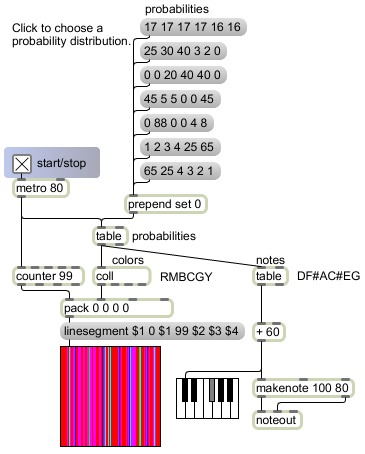
The table labeled "probabilities" stores a probability distribution. Its contents can set be set to one of seven predetermined distributions stored in the message boxes labeled "probabilities", or you can draw some other probability distribution in the table's graphic editing window. (The predetermined probabilities have all been chosen so that they add up to 100, so that the values can be thought of as percentages, but they really are meaningful relative to each other, and don't have to add up to 100.) The metro object sends bang messages to the table at a rate of 12.5 per second (once every 80 milliseconds) to make a probabilistic choice. The table object responds by sending out an index number from 0 to 5 each time based on the stored probabilities.

Those numbers are in turn treated as indices to look up the desired color and pitch events. The colors are stored in a coll object and the pitch classes are stored in another table object. This illustrates two different uses of table objects; one is used as a probability vector, and the other is used as a lookup array. The pitch choices are just stored as pitch classes 2 6 9 1 4 7 (D F# A C# E G), and those are added to the constant number 60 to transpose them into the middle octave of the piano. The color choices are stored as RGB values representing Red Magenta Blue Cyan Green Yellow, and those are drawn as vertical colored lines moving progressively from left to right. In this way one sees the distribution of probabilistic decisions as a field of colored lines, and one hears it as a sort of harmonic sonority.

The metro object, in addition to triggering a probabilistic choice in the table object, triggers the counter object to send out a number progressing from 0 to 99 indicating the horizontal offset of the colored line. That number is packed together with the color information from the coll, for use in a linesegment drawing instruction for the lcd.

Now that we've seen an explanation of discrete probability distribution, and seen how it can be implemented in a program, and seen a very simple example of how it can be applied, let's make some crucial observations about this method of decision making.

1) This technique allows us to describe a statistical distribution that characterizes a body of choices, but each individual choice is still arbitrary within those constrictions.

2) The choices are not only arbitrarily made, they produce abstract events (index numbers) that could potentially refer to anything. The actual pitch and color event possibilities were chosen carefully by the programmer to create specific sets of distinct possibilities, and the probability distributions were designed to highlight certain relationships inherent in those sets. Theoretically, though, the method of selection and the content are independent; choices are made to fulfill a statistical imperative, potentially with no regard to the eventual content of the events that those numbers will trigger.

3) Each individual choice is made ignorant of what has come before, thus there is no control over the transition from one choice to the next, thus there is no controlled sense of melody or contour in the pitch choices (other than the constraints imposed by the limited number of possibilities), nor pattern to the juxtaposition of colors. This limitation can be addressed by using a matrix of transition probabilities, known as a Markov chain, which will be demonstrated in another lesson.

4) The transitions from one probability distribution to another are all sudden rather than nuanced or gradual. This can be addressed by interpolating between distributions, which will also be demonstrated in another lesson.

5) Decision making in this example, as in most of the previous examples, is applied to only one parameter -- color in the visual domain and pitch class in the musical domain. Obviously a more interesting aesthetic result can be achieved by varying a greater number of parameters, either systematically or probabilistically. Synchronous decision making applied to many parameters at once can lead to interesting musical and visual results. This, too, is a topic for a future lesson.

A simple probabilistic decision

In all of the examples of autonomous computer decision making presented up to this point, we've used equal probabilities for all the possible choices, using the random object or its audio counterpart noise~. The resultant choices have thus been truly arbitrary, within the limits prescribed by the program.

It's also possible to use random number generation to enact decisions that are still arbitrary but are somewhat more predictable than plain randomness. One can apply a probability factor to make one choice more likely than another in a binary decision, or (as will be demonstrated in a future lesson) one can apply a more complicated probability function to a set of possibilities, giving each one a different likelihood. This lesson will demonstrate the first case, using a probability factor to make a binary decision in which one result is more likely to occur than the other.

As described briefly in an earlier lesson on randomness, the probability of a particular looked-for event occurring can be defined as a number between 0 and 1 inclusive, with that number being the ratio of the number of looked-for outcomes divided by the number of all possible outcomes. For example, the probability of choosing the the ace of spades (1 unique looked-for result) out of all possible cards in a deck (52 of them) is 1/52, which is 0.019231. The probability of not choosing the ace of spades is 1 minus that, which is 0.980769 (51/52). Thus we can say that the likelihood of choosing the ace of spades at random from a deck of cards is less than 2%, and the likelihood of not choosing it is a bit more than 98%; other ways of stating this are to say that there is a 1 in 52 chance of getting the ace of spades, or to say that the odds against choosing the ace of spades are 51 to 1.

For making an automated decision between two things, we can emulate this sort of odds by applying a probability factor between 0 and 1 to one of the choices. For example, if we want to make a decision between A and B, with both being equally likely, we would set the probability of A to 0.5 (and thus the probability of B would implicitly be 1 minus 0.5, which also equals 0.5). If we want to make A somewhat more likely than B, we could set the probability of A to something greater than 0.5, such as 0.75. This would mean there is a 75% chance of choosing A, and a 25% chance of choosing B; the odds in favor of choosing A are 3 to 1 (75:25). This does not ensure that A will always be chosen exactly thrice as many times as B. It does mean, however, that as the number of choices increases, statistically the percentage of A choices will tend toward being three times that of B.

The simplest way to do this in a computer program is as follows: Set the probability P for choice A. Choose a random number x between 0 and 1 (more specifically, 0 to just less than 1). If x is less than P, then choose A; otherwise, choose B. The result of such a program will be that over the course of numerous choices, the distribution of A choices over the total number of choices will tend toward P. The choices will still be arbitrary, and we can't predict any individual choice with certainty (unless the probability of A is either 0 or 1), but we can characterize the statistical probability of choosing A or B.

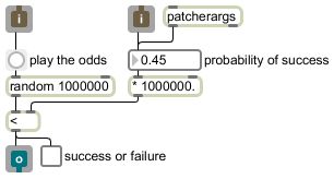
Because the random generator in Max produces whole numbers less than the specified maximum rather than fractional numbers between 0 and 1, we have to do one additional step: we either have to map the range of random numbers into the fractional 0-to-1 range, or we have to map the probability factor into the range of whole numbers. It turns out to be slightly more efficient to do the latter, because it requires doing just one multiplication when we specify the probability, rather than doing a division every time we generate a random number. The following tiny program does just that. Every time it receives a message in its inlet, it will make a probabilistic choice between two possible results, based on a provided probability factor.

The probability value that goes into the number box (either by entering the number directly or by it coming from the right inlet or the patcherargs obejct) gets multiplied by 1,000,000 and the result is stored in the right inlet of the less than object. The bang from the button (triggered either by a mouse click or by a message coming in the left inlet) causes random to generate a random number from 0 to 999,999. If it is less than the number that came from the probability factor (which would be 450,000 in the above example), it sends out a 1, otherwise it sends out a 0. You can see that statistically, over the course of many repetitions, it will tend to send out 1 about 45% of the time.

A useful programming trick that is invisible in this picture is that the number box has been set to have a minimum value of 0 and a maximum value of 1. Any value that comes in its inlet will be clipped to that range before being sent out, so the number box actually serves to limit the range and prevent any inappropriate probability values that might cause the program to malfunction. Protecting against expected or unwanted values, either from a user or from another part of the program, is good safe programming practice.

As was mentioned earlier, the multiplication of the probability by 1,000,000 is because we want to express the probability as a fraction from 0 to 1, but random only generates random whole numbers, so we need to reconcile those two ranges. We chose the number 1,000,000 because that means that we can express the probability to as many as six decimal places, and when we multiply it by 1,000,000 the result will always be a unique integer representing one of those 1,000,001 possible values (from 0.000000 to 1.000000 inclusive). Since six decimal places is the greatest precision that can be entered into a standard Max object, this program takes full advantage of the precision available in Max. It's inconceivable that you could create a situation in which you could ever hear the difference between a 0.749999 probability and a 0.750000 probability (indeed, in most musical situations it's doubtful you could even hear the difference between a 0.74 probability and a 0.75 probability), but there's no reason not to take advantage of that available precision.

Notice that this little program has been written in such a way that it can be tried out with the user interface objects number box, button, and toggle, but it was actually designed to be useful as a subpatch in some other patch, thanks to the inclusion of the inlet, outlet, and patcherargs objects. All of its input and output is actually expected to come from and go to someplace else in the parent patch, for use in a larger program. The number box clips any probability value to the 0-to-1 range, and the button converts any message in the left inlet to a bang for random. Save this patch with the name gamble, because it is used in the next example patch.

Now that we have a program that reliably makes a probabilistic decision, we'll use it to make a simple binary decision whether to play a note or not.

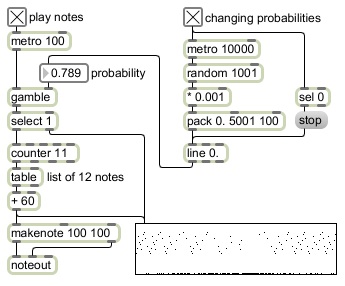
If the metro 100 object were connected directly to the counter 11 object, the patch would repeatedly count from 0 to 11, to cycle through a list of twelve pitch classes stored in the table, to play a loop at the rate of ten notes per second. However, as it is, the metro 100 object triggers the gamble object to make a probabilistic decision, 1 or 0. The select 1 object triggers a note only if the choice made by gamble is 1. If you click on the toggle to turn on the metro 100 object you will initially hear nothing because the probability of gamble choosing a 1 is set to 0. If you change the probability value to 1., gamble will always choose 1, and you will hear all the notes being played.

If the probability is set to some value in between 0 and 1, say 0.8, gamble will, on average, choose to play a note 80% of the time and choose to rest 20% of the time. The exact rhythm is unpredictable, but the average density of notes per second will be 8.

The upper right part of the patch randomly chooses a new probability somewhere in the range from 0 to 1 every ten seconds, and uses linear interpolation to arrive at the newly chosen probability value in five seconds. The probability will then stay at that new value for five seconds before the next value is chosen. By turning on this control portion of the patch, you can hear the effect of different statistical note densities in time, and the gradual transition from one density to another over five seconds.

Note that when gamble chooses 0, no note is played but the select 1 object still sends the 0 to the multislider (but not to the counter) so that the musical rest is shown in the graphic display, creating the proper depiction of the note density.

In this lesson we made a useful subpatch for making probabilistic decisions, and we used those decisions to choose whether to play a note or not. Of course the decision could be between any two things. For example you might use it to make control decisions, at a slower rate, choosing whether to run one part of the program or another, to control a longer-term formal structure.